> ## Documentation Index
> Fetch the complete documentation index at: https://docs.wandb.ai/llms.txt
> Use this file to discover all available pages before exploring further.
# PyTorch
> Integrate W&B with PyTorch for experiment tracking, dataset versioning, and logging of metrics, gradients, and models.
export const ColabLink = ({url}) =>
Try in Colab
;
Use [W\&B](https://wandb.ai) for machine learning experiment tracking, dataset versioning, and project collaboration.
## What this notebook covers
We show you how to integrate W\&B with your PyTorch code to add experiment tracking to your pipeline.
```python theme={null}
# import the library
import wandb
# capture a dictionary of hyperparameters with config
config = {
"learning_rate": 0.001,
"epochs": 100,
"batch_size": 128
}
# start a new experiment
with wandb.init(project="new-sota-model", config=config) as run:
# set up model and data
model, dataloader = get_model(), get_data()
# optional: track gradients
run.watch(model)
for batch in dataloader:
metrics = model.training_step()
# log metrics inside your training loop to visualize model performance
run.log(metrics)
# optional: save model at the end
model.to_onnx()
run.save("model.onnx")
```
Follow along with a [video tutorial](https://wandb.me/pytorch-video).
**Note**: Sections starting with *Step* are all you need to integrate W\&B in an existing pipeline. The rest just loads data and defines a model.
## Install, import, and log in
```python theme={null}
import os
import random
import numpy as np
import torch
import torch.nn as nn
import torchvision
import torchvision.transforms as transforms
from tqdm.auto import tqdm
# Ensure deterministic behavior
torch.backends.cudnn.deterministic = True
random.seed(hash("setting random seeds") % 2**32 - 1)
np.random.seed(hash("improves reproducibility") % 2**32 - 1)
torch.manual_seed(hash("by removing stochasticity") % 2**32 - 1)
torch.cuda.manual_seed_all(hash("so runs are repeatable") % 2**32 - 1)
# Device configuration
device = torch.device("cuda:0" if torch.cuda.is_available() else "cpu")
# remove slow mirror from list of MNIST mirrors
torchvision.datasets.MNIST.mirrors = [mirror for mirror in torchvision.datasets.MNIST.mirrors
if not mirror.startswith("http://yann.lecun.com")]
```
### Step 0: Install W\&B
To get started, we'll need to get the library.
`wandb` is easily installed using `pip`.
```python theme={null}
!pip install wandb onnx -Uq
```
### Step 1: Import W\&B and Login
In order to log data to our web service,
you'll need to log in.
If this is your first time using W\&B,
you'll need to sign up for a free account at the link that appears.
```
import wandb
wandb.login()
```
## Define the experiment and pipeline
### Track metadata and hyperparameters with `wandb.init()`
Programmatically, the first thing we do is define our experiment:
what are the hyperparameters? what metadata is associated with this run?
It's a pretty common workflow to store this information in a `config` dictionary
(or similar object)
and then access it as needed.
For this example, we're only letting a few hyperparameters vary
and hand-coding the rest.
But any part of your model can be part of the `config`.
We also include some metadata: we're using the MNIST dataset and a convolutional
architecture. If we later work with, say,
fully connected architectures on CIFAR in the same project,
this will help us separate our runs.
```python theme={null}
config = dict(
epochs=5,
classes=10,
kernels=[16, 32],
batch_size=128,
learning_rate=0.005,
dataset="MNIST",
architecture="CNN")
```
Now, let's define the overall pipeline,
which is pretty typical for model-training:
1. we first `make` a model, plus associated data and optimizer, then
2. we `train` the model accordingly and finally
3. `test` it to see how training went.
We'll implement these functions below.
```python theme={null}
def model_pipeline(hyperparameters):
# tell wandb to get started
with wandb.init(project="pytorch-demo", config=hyperparameters) as run:
# access all HPs through run.config, so logging matches execution.
config = run.config
# make the model, data, and optimization problem
model, train_loader, test_loader, criterion, optimizer = make(config)
print(model)
# and use them to train the model
train(model, train_loader, criterion, optimizer, config)
# and test its final performance
test(model, test_loader)
return model
```
The only difference here from a standard pipeline
is that it all occurs inside the context of `wandb.init()`.
Calling this function sets up a line of communication
between your code and our servers.
Passing the `config` dictionary to `wandb.init()`
immediately logs all that information to us,
so you'll always know what hyperparameter values
you set your experiment to use.
To ensure the values you chose and logged are always the ones that get used
in your model, we recommend using the `run.config` copy of your object.
Check the definition of `make` below to see some examples.
> *Side Note*: We take care to run our code in separate processes,
> so that any issues on our end
> (such as if a giant sea monster attacks our data centers)
> don't crash your code.
> Once the issue is resolved, such as when the Kraken returns to the deep,
> you can log the data with `wandb sync`.
```python theme={null}
def make(config):
# Make the data
train, test = get_data(train=True), get_data(train=False)
train_loader = make_loader(train, batch_size=config.batch_size)
test_loader = make_loader(test, batch_size=config.batch_size)
# Make the model
model = ConvNet(config.kernels, config.classes).to(device)
# Make the loss and optimizer
criterion = nn.CrossEntropyLoss()
optimizer = torch.optim.Adam(
model.parameters(), lr=config.learning_rate)
return model, train_loader, test_loader, criterion, optimizer
```
### Define the data loading and model
Now, we need to specify how the data is loaded and what the model looks like.
This part is very important, but it's
no different from what it would be without `wandb`,
so we won't dwell on it.
```python theme={null}
def get_data(slice=5, train=True):
full_dataset = torchvision.datasets.MNIST(root=".",
train=train,
transform=transforms.ToTensor(),
download=True)
# equiv to slicing with [::slice]
sub_dataset = torch.utils.data.Subset(
full_dataset, indices=range(0, len(full_dataset), slice))
return sub_dataset
def make_loader(dataset, batch_size):
loader = torch.utils.data.DataLoader(dataset=dataset,
batch_size=batch_size,
shuffle=True,
pin_memory=True, num_workers=2)
return loader
```
Defining the model is normally the fun part.
But nothing changes with `wandb`,
so we're gonna stick with a standard ConvNet architecture.
Don't be afraid to mess around with this and try some experiments --
all your results will be logged on [wandb.ai](https://wandb.ai).
```python theme={null}
# Conventional and convolutional neural network
class ConvNet(nn.Module):
def __init__(self, kernels, classes=10):
super(ConvNet, self).__init__()
self.layer1 = nn.Sequential(
nn.Conv2d(1, kernels[0], kernel_size=5, stride=1, padding=2),
nn.ReLU(),
nn.MaxPool2d(kernel_size=2, stride=2))
self.layer2 = nn.Sequential(
nn.Conv2d(16, kernels[1], kernel_size=5, stride=1, padding=2),
nn.ReLU(),
nn.MaxPool2d(kernel_size=2, stride=2))
self.fc = nn.Linear(7 * 7 * kernels[-1], classes)
def forward(self, x):
out = self.layer1(x)
out = self.layer2(out)
out = out.reshape(out.size(0), -1)
out = self.fc(out)
return out
```
### Define training logic
Moving on in our `model_pipeline`, it's time to specify how we `train`.
Two `wandb` functions come into play here: `watch` and `log`.
## Track gradients with `run.watch()` and everything else with `run.log()`
`run.watch()` will log the gradients and the parameters of your model,
every `log_freq` steps of training.
All you need to do is call it before you start training.
The rest of the training code remains the same:
we iterate over epochs and batches,
running forward and backward passes
and applying our `optimizer`.
```python theme={null}
def train(model, loader, criterion, optimizer, config):
# Tell wandb to watch what the model gets up to: gradients, weights, and more.
run = wandb.init(project="pytorch-demo", config=config)
run.watch(model, criterion, log="all", log_freq=10)
# Run training and track with wandb
total_batches = len(loader) * config.epochs
example_ct = 0 # number of examples seen
batch_ct = 0
for epoch in tqdm(range(config.epochs)):
for _, (images, labels) in enumerate(loader):
loss = train_batch(images, labels, model, optimizer, criterion)
example_ct += len(images)
batch_ct += 1
# Report metrics every 25th batch
if ((batch_ct + 1) % 25) == 0:
train_log(loss, example_ct, epoch)
def train_batch(images, labels, model, optimizer, criterion):
images, labels = images.to(device), labels.to(device)
# Forward pass ➡
outputs = model(images)
loss = criterion(outputs, labels)
# Backward pass ⬅
optimizer.zero_grad()
loss.backward()
# Step with optimizer
optimizer.step()
return loss
```
The only difference is in the logging code:
where previously you might have reported metrics by printing to the terminal,
now you pass the same information to `run.log()`.
`run.log()` expects a dictionary with strings as keys.
These strings identify the objects being logged, which make up the values.
You can also optionally log which `step` of training you're on.
> *Side Note*: I like to use the number of examples the model has seen,
> since this makes for easier comparison across batch sizes,
> but you can use raw steps or batch count. For longer training runs, it can also make sense to log by `epoch`.
```python theme={null}
def train_log(loss, example_ct, epoch):
with wandb.init(project="pytorch-demo") as run:
# Log the loss and epoch number
# This is where we log the metrics to W&B
run.log({"epoch": epoch, "loss": loss}, step=example_ct)
print(f"Loss after {str(example_ct).zfill(5)} examples: {loss:.3f}")
```
### Define testing logic
Once the model is done training, we want to test it:
run it against some fresh data from production, perhaps,
or apply it to some hand-curated examples.
## (Optional) Call `run.save()`
This is also a great time to save the model's architecture
and final parameters to disk.
For maximum compatibility, we'll `export` our model in the
[Open Neural Network eXchange (ONNX) format](https://onnx.ai/).
Passing that filename to `run.save()` ensures that the model parameters
are saved to W\&B's servers: no more losing track of which `.h5` or `.pb`
corresponds to which training runs.
For more advanced `wandb` features for storing, versioning, and distributing
models, check out our [Artifacts tools](https://www.wandb.com/artifacts).
```python theme={null}
def test(model, test_loader):
model.eval()
with wandb.init(project="pytorch-demo") as run:
# Run the model on some test examples
with torch.no_grad():
correct, total = 0, 0
for images, labels in test_loader:
images, labels = images.to(device), labels.to(device)
outputs = model(images)
_, predicted = torch.max(outputs.data, 1)
total += labels.size(0)
correct += (predicted == labels).sum().item()
print(f"Accuracy of the model on the {total} " +
f"test images: {correct / total:%}")
run.log({"test_accuracy": correct / total})
# Save the model in the exchangeable ONNX format
torch.onnx.export(model, images, "model.onnx")
run.save("model.onnx")
```
### Run training and watch your metrics live on wandb.ai
Now that we've defined the whole pipeline and slipped in
those few lines of W\&B code,
we're ready to run our fully tracked experiment.
We'll report a few links to you:
our documentation,
the Project page, which organizes all the runs in a project, and
the Run page, where this run's results will be stored.
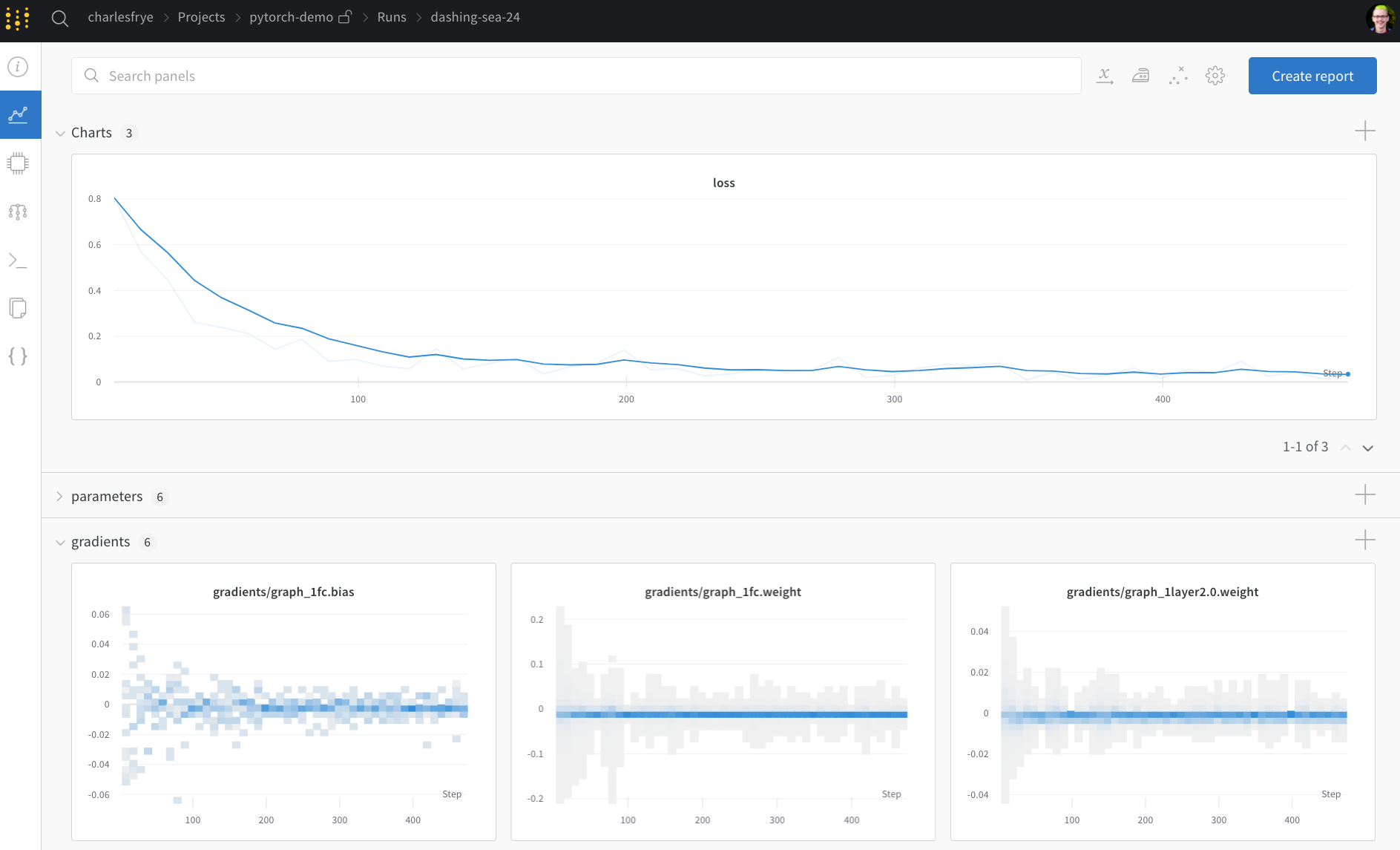
Navigate to the Run page and check out these tabs:
1. **Charts**, where the model gradients, parameter values, and loss are logged throughout training
2. **System**, which contains a variety of system metrics, including Disk I/O utilization, CPU and GPU metrics (watch that temperature soar), and more
3. **Logs**, which has a copy of anything pushed to standard out during training
4. **Files**, where, once training is complete, you can click on the `model.onnx` to view our network with the [Netron model viewer](https://github.com/lutzroeder/netron).
Once the run in finished, when the `with wandb.init()` block exits,
we'll also print a summary of the results in the cell output.
```python theme={null}
# Build, train and analyze the model with the pipeline
model = model_pipeline(config)
```
### Test Hyperparameters with Sweeps
We only looked at a single set of hyperparameters in this example.
But an important part of most ML workflows is iterating over
a number of hyperparameters.
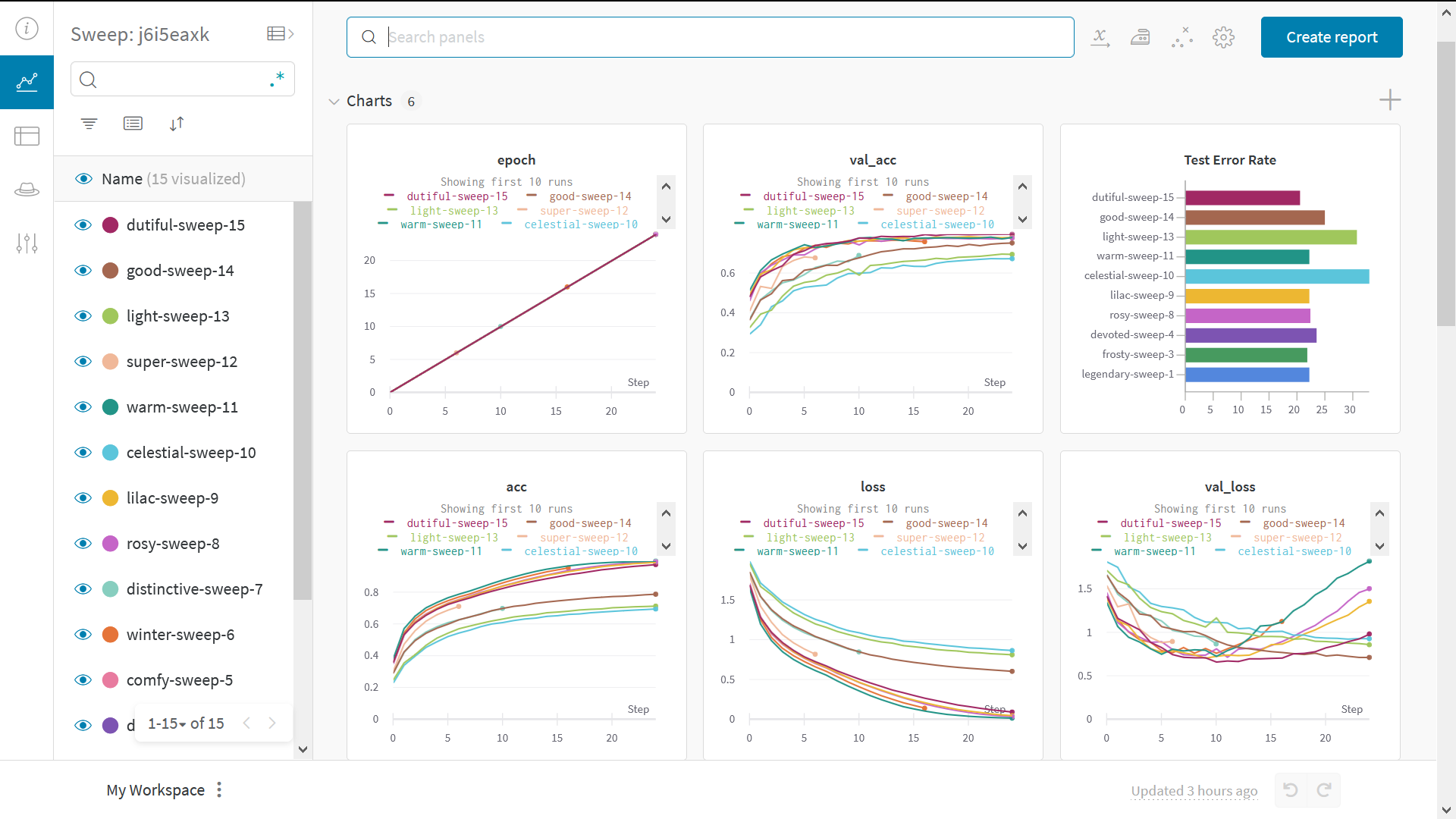
You can use W\&B Sweeps to automate hyperparameter testing and explore the space of possible models and optimization strategies.
Check out a [Colab notebook demonstrating hyperparameter optimization using W\&B Sweeps](https://wandb.me/sweeps-colab).
Running a hyperparameter sweep with W\&B is very easy. There are just 3 simple steps:
1. **Define the sweep:** We do this by creating a dictionary or a [YAML file](/models/sweeps/define-sweep-configuration/) that specifies the parameters to search through, the search strategy, the optimization metric et all.
2. **Initialize the sweep:**
`sweep_id = wandb.sweep(sweep_config)`
3. **Run the sweep agent:**
`wandb.agent(sweep_id, function=train)`
That's all there is to running a hyperparameter sweep.
## Example gallery
Explore examples of projects tracked and visualized with W\&B in our [Gallery →](https://app.wandb.ai/gallery).
## Advanced setup
1. [Environment variables](/platform/hosting/env-vars/): Set API keys in environment variables so you can run training on a managed cluster.
2. [Offline mode](/support/models/articles/how-do-i-run-wandb-offline): Use `dryrun` mode to train offline and sync results later.
3. [On-prem](/platform/hosting/hosting-options/self-managed): Install W\&B in a private cloud or air-gapped servers in your own infrastructure. We have local installations for everyone from academics to enterprise teams.
4. [Sweeps](/models/sweeps/): Set up hyperparameter search quickly with our lightweight tool for tuning.
 ## What this notebook covers
We show you how to integrate W\&B with your PyTorch code to add experiment tracking to your pipeline.
## What this notebook covers
We show you how to integrate W\&B with your PyTorch code to add experiment tracking to your pipeline.
 ```python theme={null}
# import the library
import wandb
# capture a dictionary of hyperparameters with config
config = {
"learning_rate": 0.001,
"epochs": 100,
"batch_size": 128
}
# start a new experiment
with wandb.init(project="new-sota-model", config=config) as run:
# set up model and data
model, dataloader = get_model(), get_data()
# optional: track gradients
run.watch(model)
for batch in dataloader:
metrics = model.training_step()
# log metrics inside your training loop to visualize model performance
run.log(metrics)
# optional: save model at the end
model.to_onnx()
run.save("model.onnx")
```
Follow along with a [video tutorial](https://wandb.me/pytorch-video).
**Note**: Sections starting with *Step* are all you need to integrate W\&B in an existing pipeline. The rest just loads data and defines a model.
## Install, import, and log in
```python theme={null}
import os
import random
import numpy as np
import torch
import torch.nn as nn
import torchvision
import torchvision.transforms as transforms
from tqdm.auto import tqdm
# Ensure deterministic behavior
torch.backends.cudnn.deterministic = True
random.seed(hash("setting random seeds") % 2**32 - 1)
np.random.seed(hash("improves reproducibility") % 2**32 - 1)
torch.manual_seed(hash("by removing stochasticity") % 2**32 - 1)
torch.cuda.manual_seed_all(hash("so runs are repeatable") % 2**32 - 1)
# Device configuration
device = torch.device("cuda:0" if torch.cuda.is_available() else "cpu")
# remove slow mirror from list of MNIST mirrors
torchvision.datasets.MNIST.mirrors = [mirror for mirror in torchvision.datasets.MNIST.mirrors
if not mirror.startswith("http://yann.lecun.com")]
```
### Step 0: Install W\&B
To get started, we'll need to get the library.
`wandb` is easily installed using `pip`.
```python theme={null}
!pip install wandb onnx -Uq
```
### Step 1: Import W\&B and Login
In order to log data to our web service,
you'll need to log in.
If this is your first time using W\&B,
you'll need to sign up for a free account at the link that appears.
```
import wandb
wandb.login()
```
## Define the experiment and pipeline
### Track metadata and hyperparameters with `wandb.init()`
Programmatically, the first thing we do is define our experiment:
what are the hyperparameters? what metadata is associated with this run?
It's a pretty common workflow to store this information in a `config` dictionary
(or similar object)
and then access it as needed.
For this example, we're only letting a few hyperparameters vary
and hand-coding the rest.
But any part of your model can be part of the `config`.
We also include some metadata: we're using the MNIST dataset and a convolutional
architecture. If we later work with, say,
fully connected architectures on CIFAR in the same project,
this will help us separate our runs.
```python theme={null}
config = dict(
epochs=5,
classes=10,
kernels=[16, 32],
batch_size=128,
learning_rate=0.005,
dataset="MNIST",
architecture="CNN")
```
Now, let's define the overall pipeline,
which is pretty typical for model-training:
1. we first `make` a model, plus associated data and optimizer, then
2. we `train` the model accordingly and finally
3. `test` it to see how training went.
We'll implement these functions below.
```python theme={null}
def model_pipeline(hyperparameters):
# tell wandb to get started
with wandb.init(project="pytorch-demo", config=hyperparameters) as run:
# access all HPs through run.config, so logging matches execution.
config = run.config
# make the model, data, and optimization problem
model, train_loader, test_loader, criterion, optimizer = make(config)
print(model)
# and use them to train the model
train(model, train_loader, criterion, optimizer, config)
# and test its final performance
test(model, test_loader)
return model
```
The only difference here from a standard pipeline
is that it all occurs inside the context of `wandb.init()`.
Calling this function sets up a line of communication
between your code and our servers.
Passing the `config` dictionary to `wandb.init()`
immediately logs all that information to us,
so you'll always know what hyperparameter values
you set your experiment to use.
To ensure the values you chose and logged are always the ones that get used
in your model, we recommend using the `run.config` copy of your object.
Check the definition of `make` below to see some examples.
> *Side Note*: We take care to run our code in separate processes,
> so that any issues on our end
> (such as if a giant sea monster attacks our data centers)
> don't crash your code.
> Once the issue is resolved, such as when the Kraken returns to the deep,
> you can log the data with `wandb sync`.
```python theme={null}
def make(config):
# Make the data
train, test = get_data(train=True), get_data(train=False)
train_loader = make_loader(train, batch_size=config.batch_size)
test_loader = make_loader(test, batch_size=config.batch_size)
# Make the model
model = ConvNet(config.kernels, config.classes).to(device)
# Make the loss and optimizer
criterion = nn.CrossEntropyLoss()
optimizer = torch.optim.Adam(
model.parameters(), lr=config.learning_rate)
return model, train_loader, test_loader, criterion, optimizer
```
### Define the data loading and model
Now, we need to specify how the data is loaded and what the model looks like.
This part is very important, but it's
no different from what it would be without `wandb`,
so we won't dwell on it.
```python theme={null}
def get_data(slice=5, train=True):
full_dataset = torchvision.datasets.MNIST(root=".",
train=train,
transform=transforms.ToTensor(),
download=True)
# equiv to slicing with [::slice]
sub_dataset = torch.utils.data.Subset(
full_dataset, indices=range(0, len(full_dataset), slice))
return sub_dataset
def make_loader(dataset, batch_size):
loader = torch.utils.data.DataLoader(dataset=dataset,
batch_size=batch_size,
shuffle=True,
pin_memory=True, num_workers=2)
return loader
```
Defining the model is normally the fun part.
But nothing changes with `wandb`,
so we're gonna stick with a standard ConvNet architecture.
Don't be afraid to mess around with this and try some experiments --
all your results will be logged on [wandb.ai](https://wandb.ai).
```python theme={null}
# Conventional and convolutional neural network
class ConvNet(nn.Module):
def __init__(self, kernels, classes=10):
super(ConvNet, self).__init__()
self.layer1 = nn.Sequential(
nn.Conv2d(1, kernels[0], kernel_size=5, stride=1, padding=2),
nn.ReLU(),
nn.MaxPool2d(kernel_size=2, stride=2))
self.layer2 = nn.Sequential(
nn.Conv2d(16, kernels[1], kernel_size=5, stride=1, padding=2),
nn.ReLU(),
nn.MaxPool2d(kernel_size=2, stride=2))
self.fc = nn.Linear(7 * 7 * kernels[-1], classes)
def forward(self, x):
out = self.layer1(x)
out = self.layer2(out)
out = out.reshape(out.size(0), -1)
out = self.fc(out)
return out
```
### Define training logic
Moving on in our `model_pipeline`, it's time to specify how we `train`.
Two `wandb` functions come into play here: `watch` and `log`.
## Track gradients with `run.watch()` and everything else with `run.log()`
`run.watch()` will log the gradients and the parameters of your model,
every `log_freq` steps of training.
All you need to do is call it before you start training.
The rest of the training code remains the same:
we iterate over epochs and batches,
running forward and backward passes
and applying our `optimizer`.
```python theme={null}
def train(model, loader, criterion, optimizer, config):
# Tell wandb to watch what the model gets up to: gradients, weights, and more.
run = wandb.init(project="pytorch-demo", config=config)
run.watch(model, criterion, log="all", log_freq=10)
# Run training and track with wandb
total_batches = len(loader) * config.epochs
example_ct = 0 # number of examples seen
batch_ct = 0
for epoch in tqdm(range(config.epochs)):
for _, (images, labels) in enumerate(loader):
loss = train_batch(images, labels, model, optimizer, criterion)
example_ct += len(images)
batch_ct += 1
# Report metrics every 25th batch
if ((batch_ct + 1) % 25) == 0:
train_log(loss, example_ct, epoch)
def train_batch(images, labels, model, optimizer, criterion):
images, labels = images.to(device), labels.to(device)
# Forward pass ➡
outputs = model(images)
loss = criterion(outputs, labels)
# Backward pass ⬅
optimizer.zero_grad()
loss.backward()
# Step with optimizer
optimizer.step()
return loss
```
The only difference is in the logging code:
where previously you might have reported metrics by printing to the terminal,
now you pass the same information to `run.log()`.
`run.log()` expects a dictionary with strings as keys.
These strings identify the objects being logged, which make up the values.
You can also optionally log which `step` of training you're on.
> *Side Note*: I like to use the number of examples the model has seen,
> since this makes for easier comparison across batch sizes,
> but you can use raw steps or batch count. For longer training runs, it can also make sense to log by `epoch`.
```python theme={null}
def train_log(loss, example_ct, epoch):
with wandb.init(project="pytorch-demo") as run:
# Log the loss and epoch number
# This is where we log the metrics to W&B
run.log({"epoch": epoch, "loss": loss}, step=example_ct)
print(f"Loss after {str(example_ct).zfill(5)} examples: {loss:.3f}")
```
### Define testing logic
Once the model is done training, we want to test it:
run it against some fresh data from production, perhaps,
or apply it to some hand-curated examples.
## (Optional) Call `run.save()`
This is also a great time to save the model's architecture
and final parameters to disk.
For maximum compatibility, we'll `export` our model in the
[Open Neural Network eXchange (ONNX) format](https://onnx.ai/).
Passing that filename to `run.save()` ensures that the model parameters
are saved to W\&B's servers: no more losing track of which `.h5` or `.pb`
corresponds to which training runs.
For more advanced `wandb` features for storing, versioning, and distributing
models, check out our [Artifacts tools](https://www.wandb.com/artifacts).
```python theme={null}
def test(model, test_loader):
model.eval()
with wandb.init(project="pytorch-demo") as run:
# Run the model on some test examples
with torch.no_grad():
correct, total = 0, 0
for images, labels in test_loader:
images, labels = images.to(device), labels.to(device)
outputs = model(images)
_, predicted = torch.max(outputs.data, 1)
total += labels.size(0)
correct += (predicted == labels).sum().item()
print(f"Accuracy of the model on the {total} " +
f"test images: {correct / total:%}")
run.log({"test_accuracy": correct / total})
# Save the model in the exchangeable ONNX format
torch.onnx.export(model, images, "model.onnx")
run.save("model.onnx")
```
### Run training and watch your metrics live on wandb.ai
Now that we've defined the whole pipeline and slipped in
those few lines of W\&B code,
we're ready to run our fully tracked experiment.
We'll report a few links to you:
our documentation,
the Project page, which organizes all the runs in a project, and
the Run page, where this run's results will be stored.
Navigate to the Run page and check out these tabs:
1. **Charts**, where the model gradients, parameter values, and loss are logged throughout training
2. **System**, which contains a variety of system metrics, including Disk I/O utilization, CPU and GPU metrics (watch that temperature soar), and more
3. **Logs**, which has a copy of anything pushed to standard out during training
4. **Files**, where, once training is complete, you can click on the `model.onnx` to view our network with the [Netron model viewer](https://github.com/lutzroeder/netron).
Once the run in finished, when the `with wandb.init()` block exits,
we'll also print a summary of the results in the cell output.
```python theme={null}
# Build, train and analyze the model with the pipeline
model = model_pipeline(config)
```
### Test Hyperparameters with Sweeps
We only looked at a single set of hyperparameters in this example.
But an important part of most ML workflows is iterating over
a number of hyperparameters.
You can use W\&B Sweeps to automate hyperparameter testing and explore the space of possible models and optimization strategies.
Check out a [Colab notebook demonstrating hyperparameter optimization using W\&B Sweeps](https://wandb.me/sweeps-colab).
Running a hyperparameter sweep with W\&B is very easy. There are just 3 simple steps:
1. **Define the sweep:** We do this by creating a dictionary or a [YAML file](/models/sweeps/define-sweep-configuration/) that specifies the parameters to search through, the search strategy, the optimization metric et all.
2. **Initialize the sweep:**
`sweep_id = wandb.sweep(sweep_config)`
3. **Run the sweep agent:**
`wandb.agent(sweep_id, function=train)`
That's all there is to running a hyperparameter sweep.
```python theme={null}
# import the library
import wandb
# capture a dictionary of hyperparameters with config
config = {
"learning_rate": 0.001,
"epochs": 100,
"batch_size": 128
}
# start a new experiment
with wandb.init(project="new-sota-model", config=config) as run:
# set up model and data
model, dataloader = get_model(), get_data()
# optional: track gradients
run.watch(model)
for batch in dataloader:
metrics = model.training_step()
# log metrics inside your training loop to visualize model performance
run.log(metrics)
# optional: save model at the end
model.to_onnx()
run.save("model.onnx")
```
Follow along with a [video tutorial](https://wandb.me/pytorch-video).
**Note**: Sections starting with *Step* are all you need to integrate W\&B in an existing pipeline. The rest just loads data and defines a model.
## Install, import, and log in
```python theme={null}
import os
import random
import numpy as np
import torch
import torch.nn as nn
import torchvision
import torchvision.transforms as transforms
from tqdm.auto import tqdm
# Ensure deterministic behavior
torch.backends.cudnn.deterministic = True
random.seed(hash("setting random seeds") % 2**32 - 1)
np.random.seed(hash("improves reproducibility") % 2**32 - 1)
torch.manual_seed(hash("by removing stochasticity") % 2**32 - 1)
torch.cuda.manual_seed_all(hash("so runs are repeatable") % 2**32 - 1)
# Device configuration
device = torch.device("cuda:0" if torch.cuda.is_available() else "cpu")
# remove slow mirror from list of MNIST mirrors
torchvision.datasets.MNIST.mirrors = [mirror for mirror in torchvision.datasets.MNIST.mirrors
if not mirror.startswith("http://yann.lecun.com")]
```
### Step 0: Install W\&B
To get started, we'll need to get the library.
`wandb` is easily installed using `pip`.
```python theme={null}
!pip install wandb onnx -Uq
```
### Step 1: Import W\&B and Login
In order to log data to our web service,
you'll need to log in.
If this is your first time using W\&B,
you'll need to sign up for a free account at the link that appears.
```
import wandb
wandb.login()
```
## Define the experiment and pipeline
### Track metadata and hyperparameters with `wandb.init()`
Programmatically, the first thing we do is define our experiment:
what are the hyperparameters? what metadata is associated with this run?
It's a pretty common workflow to store this information in a `config` dictionary
(or similar object)
and then access it as needed.
For this example, we're only letting a few hyperparameters vary
and hand-coding the rest.
But any part of your model can be part of the `config`.
We also include some metadata: we're using the MNIST dataset and a convolutional
architecture. If we later work with, say,
fully connected architectures on CIFAR in the same project,
this will help us separate our runs.
```python theme={null}
config = dict(
epochs=5,
classes=10,
kernels=[16, 32],
batch_size=128,
learning_rate=0.005,
dataset="MNIST",
architecture="CNN")
```
Now, let's define the overall pipeline,
which is pretty typical for model-training:
1. we first `make` a model, plus associated data and optimizer, then
2. we `train` the model accordingly and finally
3. `test` it to see how training went.
We'll implement these functions below.
```python theme={null}
def model_pipeline(hyperparameters):
# tell wandb to get started
with wandb.init(project="pytorch-demo", config=hyperparameters) as run:
# access all HPs through run.config, so logging matches execution.
config = run.config
# make the model, data, and optimization problem
model, train_loader, test_loader, criterion, optimizer = make(config)
print(model)
# and use them to train the model
train(model, train_loader, criterion, optimizer, config)
# and test its final performance
test(model, test_loader)
return model
```
The only difference here from a standard pipeline
is that it all occurs inside the context of `wandb.init()`.
Calling this function sets up a line of communication
between your code and our servers.
Passing the `config` dictionary to `wandb.init()`
immediately logs all that information to us,
so you'll always know what hyperparameter values
you set your experiment to use.
To ensure the values you chose and logged are always the ones that get used
in your model, we recommend using the `run.config` copy of your object.
Check the definition of `make` below to see some examples.
> *Side Note*: We take care to run our code in separate processes,
> so that any issues on our end
> (such as if a giant sea monster attacks our data centers)
> don't crash your code.
> Once the issue is resolved, such as when the Kraken returns to the deep,
> you can log the data with `wandb sync`.
```python theme={null}
def make(config):
# Make the data
train, test = get_data(train=True), get_data(train=False)
train_loader = make_loader(train, batch_size=config.batch_size)
test_loader = make_loader(test, batch_size=config.batch_size)
# Make the model
model = ConvNet(config.kernels, config.classes).to(device)
# Make the loss and optimizer
criterion = nn.CrossEntropyLoss()
optimizer = torch.optim.Adam(
model.parameters(), lr=config.learning_rate)
return model, train_loader, test_loader, criterion, optimizer
```
### Define the data loading and model
Now, we need to specify how the data is loaded and what the model looks like.
This part is very important, but it's
no different from what it would be without `wandb`,
so we won't dwell on it.
```python theme={null}
def get_data(slice=5, train=True):
full_dataset = torchvision.datasets.MNIST(root=".",
train=train,
transform=transforms.ToTensor(),
download=True)
# equiv to slicing with [::slice]
sub_dataset = torch.utils.data.Subset(
full_dataset, indices=range(0, len(full_dataset), slice))
return sub_dataset
def make_loader(dataset, batch_size):
loader = torch.utils.data.DataLoader(dataset=dataset,
batch_size=batch_size,
shuffle=True,
pin_memory=True, num_workers=2)
return loader
```
Defining the model is normally the fun part.
But nothing changes with `wandb`,
so we're gonna stick with a standard ConvNet architecture.
Don't be afraid to mess around with this and try some experiments --
all your results will be logged on [wandb.ai](https://wandb.ai).
```python theme={null}
# Conventional and convolutional neural network
class ConvNet(nn.Module):
def __init__(self, kernels, classes=10):
super(ConvNet, self).__init__()
self.layer1 = nn.Sequential(
nn.Conv2d(1, kernels[0], kernel_size=5, stride=1, padding=2),
nn.ReLU(),
nn.MaxPool2d(kernel_size=2, stride=2))
self.layer2 = nn.Sequential(
nn.Conv2d(16, kernels[1], kernel_size=5, stride=1, padding=2),
nn.ReLU(),
nn.MaxPool2d(kernel_size=2, stride=2))
self.fc = nn.Linear(7 * 7 * kernels[-1], classes)
def forward(self, x):
out = self.layer1(x)
out = self.layer2(out)
out = out.reshape(out.size(0), -1)
out = self.fc(out)
return out
```
### Define training logic
Moving on in our `model_pipeline`, it's time to specify how we `train`.
Two `wandb` functions come into play here: `watch` and `log`.
## Track gradients with `run.watch()` and everything else with `run.log()`
`run.watch()` will log the gradients and the parameters of your model,
every `log_freq` steps of training.
All you need to do is call it before you start training.
The rest of the training code remains the same:
we iterate over epochs and batches,
running forward and backward passes
and applying our `optimizer`.
```python theme={null}
def train(model, loader, criterion, optimizer, config):
# Tell wandb to watch what the model gets up to: gradients, weights, and more.
run = wandb.init(project="pytorch-demo", config=config)
run.watch(model, criterion, log="all", log_freq=10)
# Run training and track with wandb
total_batches = len(loader) * config.epochs
example_ct = 0 # number of examples seen
batch_ct = 0
for epoch in tqdm(range(config.epochs)):
for _, (images, labels) in enumerate(loader):
loss = train_batch(images, labels, model, optimizer, criterion)
example_ct += len(images)
batch_ct += 1
# Report metrics every 25th batch
if ((batch_ct + 1) % 25) == 0:
train_log(loss, example_ct, epoch)
def train_batch(images, labels, model, optimizer, criterion):
images, labels = images.to(device), labels.to(device)
# Forward pass ➡
outputs = model(images)
loss = criterion(outputs, labels)
# Backward pass ⬅
optimizer.zero_grad()
loss.backward()
# Step with optimizer
optimizer.step()
return loss
```
The only difference is in the logging code:
where previously you might have reported metrics by printing to the terminal,
now you pass the same information to `run.log()`.
`run.log()` expects a dictionary with strings as keys.
These strings identify the objects being logged, which make up the values.
You can also optionally log which `step` of training you're on.
> *Side Note*: I like to use the number of examples the model has seen,
> since this makes for easier comparison across batch sizes,
> but you can use raw steps or batch count. For longer training runs, it can also make sense to log by `epoch`.
```python theme={null}
def train_log(loss, example_ct, epoch):
with wandb.init(project="pytorch-demo") as run:
# Log the loss and epoch number
# This is where we log the metrics to W&B
run.log({"epoch": epoch, "loss": loss}, step=example_ct)
print(f"Loss after {str(example_ct).zfill(5)} examples: {loss:.3f}")
```
### Define testing logic
Once the model is done training, we want to test it:
run it against some fresh data from production, perhaps,
or apply it to some hand-curated examples.
## (Optional) Call `run.save()`
This is also a great time to save the model's architecture
and final parameters to disk.
For maximum compatibility, we'll `export` our model in the
[Open Neural Network eXchange (ONNX) format](https://onnx.ai/).
Passing that filename to `run.save()` ensures that the model parameters
are saved to W\&B's servers: no more losing track of which `.h5` or `.pb`
corresponds to which training runs.
For more advanced `wandb` features for storing, versioning, and distributing
models, check out our [Artifacts tools](https://www.wandb.com/artifacts).
```python theme={null}
def test(model, test_loader):
model.eval()
with wandb.init(project="pytorch-demo") as run:
# Run the model on some test examples
with torch.no_grad():
correct, total = 0, 0
for images, labels in test_loader:
images, labels = images.to(device), labels.to(device)
outputs = model(images)
_, predicted = torch.max(outputs.data, 1)
total += labels.size(0)
correct += (predicted == labels).sum().item()
print(f"Accuracy of the model on the {total} " +
f"test images: {correct / total:%}")
run.log({"test_accuracy": correct / total})
# Save the model in the exchangeable ONNX format
torch.onnx.export(model, images, "model.onnx")
run.save("model.onnx")
```
### Run training and watch your metrics live on wandb.ai
Now that we've defined the whole pipeline and slipped in
those few lines of W\&B code,
we're ready to run our fully tracked experiment.
We'll report a few links to you:
our documentation,
the Project page, which organizes all the runs in a project, and
the Run page, where this run's results will be stored.
Navigate to the Run page and check out these tabs:
1. **Charts**, where the model gradients, parameter values, and loss are logged throughout training
2. **System**, which contains a variety of system metrics, including Disk I/O utilization, CPU and GPU metrics (watch that temperature soar), and more
3. **Logs**, which has a copy of anything pushed to standard out during training
4. **Files**, where, once training is complete, you can click on the `model.onnx` to view our network with the [Netron model viewer](https://github.com/lutzroeder/netron).
Once the run in finished, when the `with wandb.init()` block exits,
we'll also print a summary of the results in the cell output.
```python theme={null}
# Build, train and analyze the model with the pipeline
model = model_pipeline(config)
```
### Test Hyperparameters with Sweeps
We only looked at a single set of hyperparameters in this example.
But an important part of most ML workflows is iterating over
a number of hyperparameters.
You can use W\&B Sweeps to automate hyperparameter testing and explore the space of possible models and optimization strategies.
Check out a [Colab notebook demonstrating hyperparameter optimization using W\&B Sweeps](https://wandb.me/sweeps-colab).
Running a hyperparameter sweep with W\&B is very easy. There are just 3 simple steps:
1. **Define the sweep:** We do this by creating a dictionary or a [YAML file](/models/sweeps/define-sweep-configuration/) that specifies the parameters to search through, the search strategy, the optimization metric et all.
2. **Initialize the sweep:**
`sweep_id = wandb.sweep(sweep_config)`
3. **Run the sweep agent:**
`wandb.agent(sweep_id, function=train)`
That's all there is to running a hyperparameter sweep.
 ## Example gallery
Explore examples of projects tracked and visualized with W\&B in our [Gallery →](https://app.wandb.ai/gallery).
## Advanced setup
1. [Environment variables](/platform/hosting/env-vars/): Set API keys in environment variables so you can run training on a managed cluster.
2. [Offline mode](/support/models/articles/how-do-i-run-wandb-offline): Use `dryrun` mode to train offline and sync results later.
3. [On-prem](/platform/hosting/hosting-options/self-managed): Install W\&B in a private cloud or air-gapped servers in your own infrastructure. We have local installations for everyone from academics to enterprise teams.
4. [Sweeps](/models/sweeps/): Set up hyperparameter search quickly with our lightweight tool for tuning.
## Example gallery
Explore examples of projects tracked and visualized with W\&B in our [Gallery →](https://app.wandb.ai/gallery).
## Advanced setup
1. [Environment variables](/platform/hosting/env-vars/): Set API keys in environment variables so you can run training on a managed cluster.
2. [Offline mode](/support/models/articles/how-do-i-run-wandb-offline): Use `dryrun` mode to train offline and sync results later.
3. [On-prem](/platform/hosting/hosting-options/self-managed): Install W\&B in a private cloud or air-gapped servers in your own infrastructure. We have local installations for everyone from academics to enterprise teams.
4. [Sweeps](/models/sweeps/): Set up hyperparameter search quickly with our lightweight tool for tuning.