> ## Documentation Index
> Fetch the complete documentation index at: https://docs.wandb.ai/llms.txt
> Use this file to discover all available pages before exploring further.
> Log rich media, from 3D point clouds and molecules to HTML and histograms
# Log media and objects
export const ColabLink = ({url}) =>
Try in Colab
;
We support images, video, audio, and more. Log rich media to explore your results and visually compare your runs, models, and datasets. Read on for examples and how-to guides.
For details, see the [Data types reference](/models/ref/python/data-types/).
For more details, check out a [demo report about visualize model predictions](https://wandb.ai/lavanyashukla/visualize-predictions/reports/Visualize-Model-Predictions--Vmlldzo1NjM4OA) or watch a [video walkthrough](https://www.youtube.com/watch?v=96MxRvx15Ts).
## Pre-requisites
In order to log media objects with the W\&B SDK, you may need to install additional dependencies.
You can install these dependencies by running the following command:
```bash theme={null}
pip install wandb[media]
```
## Images
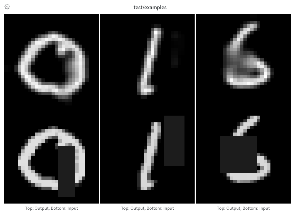
Log images to track inputs, outputs, filter weights, activations, and more.
Images can be logged directly from NumPy arrays, as PIL images, or from the filesystem.
Each time you log images from a step, they are available in the UI. Expand the image panel, then use the step slider to look at images from different steps. This makes it easy to compare how a model's output changes during training. Click a media panel to view an image in full-screen mode; there you can zoom and pan, including with [keyboard shortcuts](/models/app/keyboard-shortcuts#media-panels).
To compare images or videos from different runs, steps, or indices in one view, use [Compare mode](/models/app/features/panels/media#compare-mode) in a media panel.
It's recommended to log fewer than 50 images per step to prevent logging from becoming a bottleneck during training and image loading from becoming a bottleneck when viewing results.
Provide arrays directly when constructing images manually, such as by using [`make_grid` from `torchvision`](https://pytorch.org/vision/stable/utils.html#torchvision.utils.make_grid).
Arrays are converted to png using [Pillow](https://pillow.readthedocs.io/en/stable/index.html).
```python theme={null}
import wandb
with wandb.init(project="image-log-example") as run:
images = wandb.Image(image_array, caption="Top: Output, Bottom: Input")
run.log({"examples": images})
```
We assume the image is gray scale if the last dimension is 1, RGB if it's 3, and RGBA if it's 4. If the array contains floats, we convert them to integers between `0` and `255`. If you want to normalize your images differently, you can specify the [`mode`](https://pillow.readthedocs.io/en/stable/handbook/concepts.html#modes) manually or just supply a [`PIL.Image`](https://pillow.readthedocs.io/en/stable/reference/Image.html), as described in the "Logging PIL Images" tab of this panel.
For full control over the conversion of arrays to images, construct the [`PIL.Image`](https://pillow.readthedocs.io/en/stable/reference/Image.html) yourself and provide it directly.
```python theme={null}
from PIL import Image
with wandb.init(project="") as run:
# Create a PIL image from a NumPy array
image = Image.fromarray(image_array)
# Optionally, convert to RGB if needed
if image.mode != "RGB":
image = image.convert("RGB")
# Log the image
run.log({"example": wandb.Image(image, caption="My Image")})
```
For even more control, create images however you like, save them to disk, and provide a filepath.
```python theme={null}
import wandb
from PIL import Image
with wandb.init(project="") as run:
im = Image.fromarray(...)
rgb_im = im.convert("RGB")
rgb_im.save("myimage.jpg")
run.log({"example": wandb.Image("myimage.jpg")})
```
## Image overlays
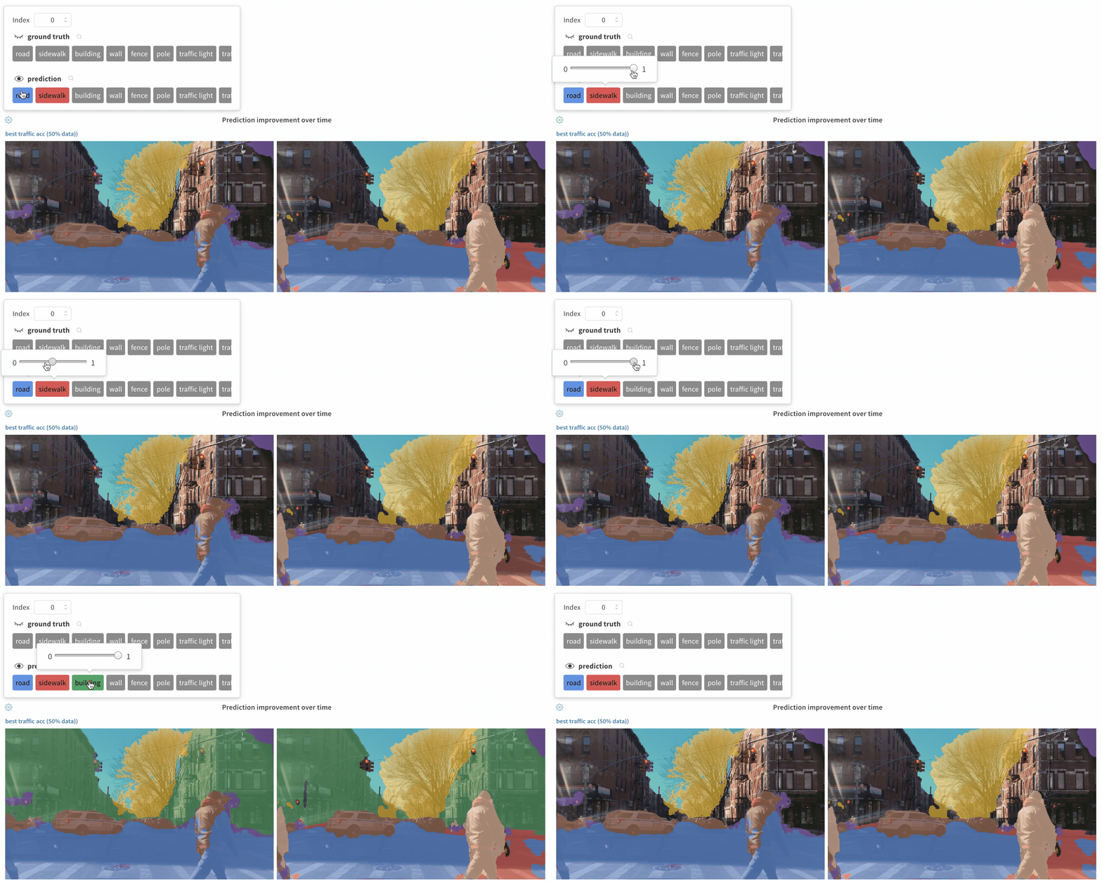
Log semantic segmentation masks and interact with them (altering opacity, viewing changes over time, and more) via the W\&B UI.
To log an overlay, provide a dictionary with the following keys and values to the `masks` keyword argument of `wandb.Image`:
* one of two keys representing the image mask:
* `"mask_data"`: a 2D NumPy array containing an integer class label for each pixel
* `"path"`: (string) a path to a saved image mask file
* `"class_labels"`: (optional) a dictionary mapping the integer class labels in the image mask to their readable class names
To log multiple masks, log a mask dictionary with multiple keys, as in the code snippet below.
[See a live example](https://app.wandb.ai/stacey/deep-drive/reports/Image-Masks-for-Semantic-Segmentation--Vmlldzo4MTUwMw)
[Sample code](https://colab.research.google.com/drive/1SOVl3EvW82Q4QKJXX6JtHye4wFix_P4J)
```python theme={null}
mask_data = np.array([[1, 2, 2, ..., 2, 2, 1], ...])
class_labels = {1: "tree", 2: "car", 3: "road"}
mask_img = wandb.Image(
image,
masks={
"predictions": {"mask_data": mask_data, "class_labels": class_labels},
"ground_truth": {
# ...
},
# ...
},
)
```
Segmentation masks for a key are defined at each step (each call to `run.log()`).
* If steps provide different values for the same mask key, only the most recent value for the key is applied to the image.
* If steps provide different mask keys, all values for each key are shown, but only those defined in the step being viewed are applied to the image. Toggling the visibility of masks not defined in the step do not change the image.
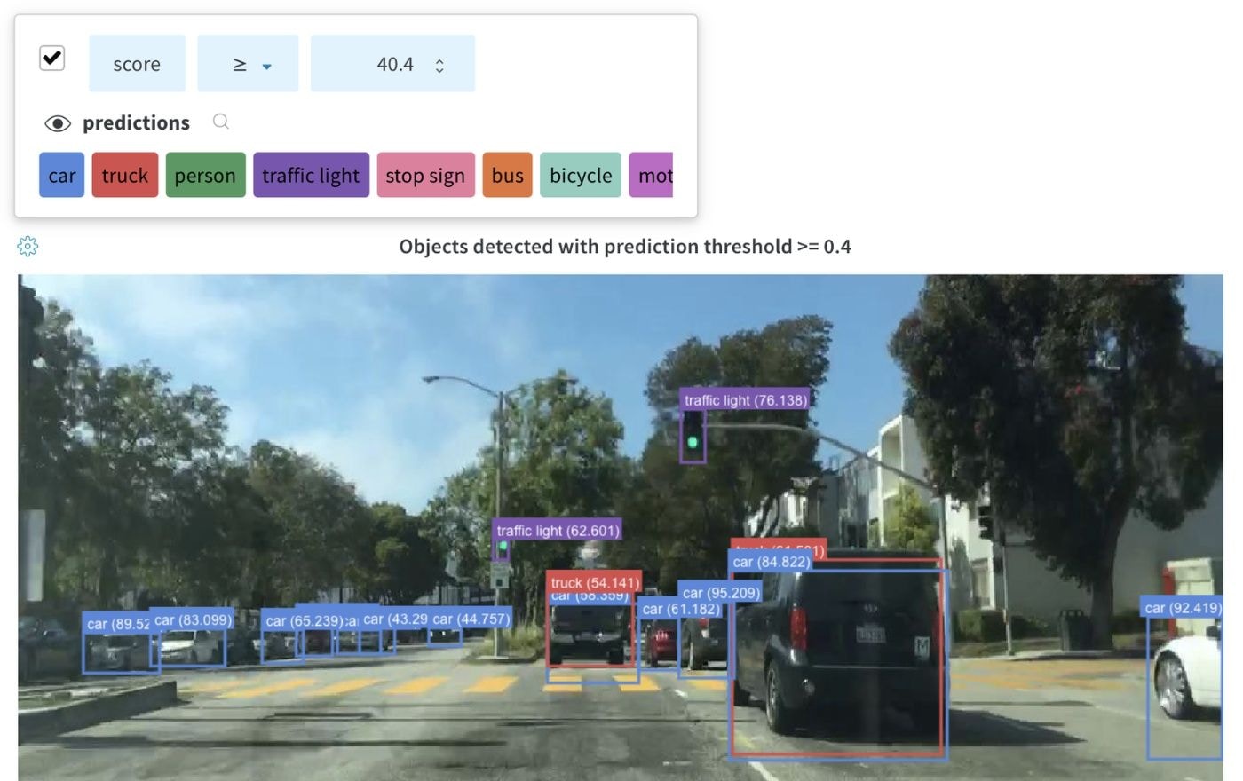
Log bounding boxes with images, and use filters and toggles to dynamically visualize different sets of boxes in the UI.
[See a live example](https://app.wandb.ai/stacey/yolo-drive/reports/Bounding-Boxes-for-Object-Detection--Vmlldzo4Nzg4MQ)
To log a bounding box, you'll need to provide a dictionary with the following keys and values to the boxes keyword argument of `wandb.Image`:
* `box_data`: a list of dictionaries, one for each box. The box dictionary format is described below.
* `position`: a dictionary representing the position and size of the box in one of two formats, as described below. Boxes need not all use the same format.
* *Option 1:* `{"minX", "maxX", "minY", "maxY"}`. Provide a set of coordinates defining the upper and lower bounds of each box dimension.
* *Option 2:* `{"middle", "width", "height"}`. Provide a set of coordinates specifying the `middle` coordinates as `[x,y]`, and `width` and `height` as scalars.
* `class_id`: an integer representing the class identity of the box. See `class_labels` key below.
* `scores`: a dictionary of string labels and numeric values for scores. Can be used for filtering boxes in the UI.
* `domain`: specify the units/format of the box coordinates. **Set this to "pixel"** if the box coordinates are expressed in pixel space, such as integers within the bounds of the image dimensions. By default, the domain is assumed to be a fraction/percentage of the image, expressed as a floating point number between 0 and 1.
* `box_caption`: (optional) a string to be displayed as the label text on this box
* `class_labels`: (optional) A dictionary mapping `class_id`s to strings. By default we will generate class labels `class_0`, `class_1`, etc.
Check out this example:
```python theme={null}
import wandb
class_id_to_label = {
1: "car",
2: "road",
3: "building",
# ...
}
img = wandb.Image(
image,
boxes={
"predictions": {
"box_data": [
{
# one box expressed in the default relative/fractional domain
"position": {"minX": 0.1, "maxX": 0.2, "minY": 0.3, "maxY": 0.4},
"class_id": 2,
"box_caption": class_id_to_label[2],
"scores": {"acc": 0.1, "loss": 1.2},
# another box expressed in the pixel domain
# (for illustration purposes only, all boxes are likely
# to be in the same domain/format)
"position": {"middle": [150, 20], "width": 68, "height": 112},
"domain": "pixel",
"class_id": 3,
"box_caption": "a building",
"scores": {"acc": 0.5, "loss": 0.7},
# ...
# Log as many boxes an as needed
}
],
"class_labels": class_id_to_label,
},
# Log each meaningful group of boxes with a unique key name
"ground_truth": {
# ...
},
},
)
with wandb.init(project="my_project") as run:
run.log({"driving_scene": img})
```
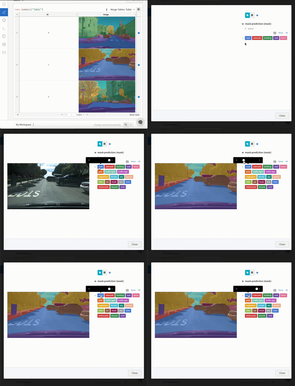
## Image overlays in Tables
To log Segmentation Masks in tables, you will need to provide a `wandb.Image` object for each row in the table.
An example is provided in the Code snippet below:
```python theme={null}
table = wandb.Table(columns=["ID", "Image"])
for id, img, label in zip(ids, images, labels):
mask_img = wandb.Image(
img,
masks={
"prediction": {"mask_data": label, "class_labels": class_labels}
# ...
},
)
table.add_data(id, mask_img)
with wandb.init(project="my_project") as run:
run.log({"Table": table})
```
To log Images with Bounding Boxes in tables, you will need to provide a `wandb.Image` object for each row in the table.
An example is provided in the code snippet below:
```python theme={null}
table = wandb.Table(columns=["ID", "Image"])
for id, img, boxes in zip(ids, images, boxes_set):
box_img = wandb.Image(
img,
boxes={
"prediction": {
"box_data": [
{
"position": {
"minX": box["minX"],
"minY": box["minY"],
"maxX": box["maxX"],
"maxY": box["maxY"],
},
"class_id": box["class_id"],
"box_caption": box["caption"],
"domain": "pixel",
}
for box in boxes
],
"class_labels": class_labels,
}
},
)
```
## Histograms
If a sequence of numbers, such as a list, array, or tensor, is provided as the first argument, we will construct the histogram automatically by calling `np.histogram()`. All arrays/tensors are flattened. You can use the optional `num_bins` keyword argument to override the default of `64` bins. The maximum number of bins supported is `512`.
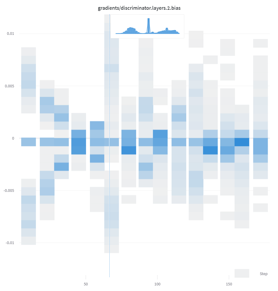
In the UI, histograms are plotted with the training step on the x-axis, the metric value on the y-axis, and the count represented by color, to ease comparison of histograms logged throughout training. See the "Histograms in Summary" tab of this panel for details on logging one-off histograms.
```python theme={null}
run.log({"gradients": wandb.Histogram(grads)})
```
If you want more control, call `np.histogram()` and pass the returned tuple to the `np_histogram` keyword argument.
```python theme={null}
np_hist_grads = np.histogram(grads, density=True, range=(0.0, 1.0))
run.log({"gradients": wandb.Histogram(np_hist_grads)})
```
If histograms are in your summary they will appear on the Overview tab of the [Run Page](/models/runs/). If they are in your history, we plot a heatmap of bins over time on the Charts tab.
## 3D visualizations
Log 3D point clouds and Lidar scenes with bounding boxes. Pass in a NumPy array containing coordinates and colors for the points to render.
```python theme={null}
point_cloud = np.array([[0, 0, 0, COLOR]])
run.log({"point_cloud": wandb.Object3D(point_cloud)})
```
The W\&B UI truncates the data at 300,000 points.
#### NumPy array formats
Three different formats of NumPy arrays are supported for flexible color schemes.
* `[[x, y, z], ...]` `nx3`
* `[[x, y, z, c], ...]` `nx4` `| c is a category` in the range `[1, 14]` (Useful for segmentation)
* `[[x, y, z, r, g, b], ...]` `nx6 | r,g,b` are values in the range `[0,255]`for red, green, and blue color channels.
#### Python object
Using this schema, you can define a Python object and pass it in to [the `from_point_cloud` method](/models/ref/python/#from_point_cloud).
* `points`is a NumPy array containing coordinates and colors for the points to render using [the same formats as the simple point cloud renderer shown above](#python-object).
* `boxes` is a NumPy array of python dictionaries with three attributes:
* `corners`- a list of eight corners
* `label`- a string representing the label to be rendered on the box (Optional)
* `color`- rgb values representing the color of the box
* `score` - a numeric value that will be displayed on the bounding box that can be used to filter the bounding boxes shown (for example, to only show bounding boxes where `score` > `0.75`). (Optional)
* `type` is a string representing the scene type to render. Currently the only supported value is `lidar/beta`
```python theme={null}
point_list = [
[
2566.571924017235, # x
746.7817289698219, # y
-15.269245470863748,# z
76.5, # red
127.5, # green
89.46617199365393 # blue
],
[ 2566.592983606823, 746.6791987335685, -15.275803826279521, 76.5, 127.5, 89.45471117247024 ],
[ 2566.616361739416, 746.4903185513501, -15.28628929674075, 76.5, 127.5, 89.41336375503832 ],
[ 2561.706014951675, 744.5349468458361, -14.877496818222781, 76.5, 127.5, 82.21868245418283 ],
[ 2561.5281847916694, 744.2546118233013, -14.867862032341005, 76.5, 127.5, 81.87824684536432 ],
[ 2561.3693562897465, 744.1804761656741, -14.854129178142523, 76.5, 127.5, 81.64137897587152 ],
[ 2561.6093071504515, 744.0287526628543, -14.882135189841177, 76.5, 127.5, 81.89871499537098 ],
# ... and so on
]
run.log({"my_first_point_cloud": wandb.Object3D.from_point_cloud(
points = point_list,
boxes = [{
"corners": [
[ 2601.2765123137915, 767.5669506323393, -17.816764802288663 ],
[ 2599.7259021588347, 769.0082337923552, -17.816764802288663 ],
[ 2599.7259021588347, 769.0082337923552, -19.66876480228866 ],
[ 2601.2765123137915, 767.5669506323393, -19.66876480228866 ],
[ 2604.8684867834395, 771.4313904894723, -17.816764802288663 ],
[ 2603.3178766284827, 772.8726736494882, -17.816764802288663 ],
[ 2603.3178766284827, 772.8726736494882, -19.66876480228866 ],
[ 2604.8684867834395, 771.4313904894723, -19.66876480228866 ]
],
"color": [0, 0, 255], # color in RGB of the bounding box
"label": "car", # string displayed on the bounding box
"score": 0.6 # numeric displayed on the bounding box
}],
vectors = [
{"start": [0, 0, 0], "end": [0.1, 0.2, 0.5], "color": [255, 0, 0]}, # color is optional
],
point_cloud_type = "lidar/beta",
)})
```
When viewing a point cloud, you can hold control and use the mouse to move around inside the space.
#### Point cloud files
You can use [the `from_file` method](/models/ref/python/#from_file) to load in a JSON file full of point cloud data.
```python theme={null}
run.log({"my_cloud_from_file": wandb.Object3D.from_file(
"./my_point_cloud.pts.json"
)})
```
An example of how to format the point cloud data is shown below.
```json theme={null}
{
"boxes": [
{
"color": [
0,
255,
0
],
"score": 0.35,
"label": "My label",
"corners": [
[
2589.695869075582,
760.7400443552185,
-18.044831294622487
],
[
2590.719039645323,
762.3871153874499,
-18.044831294622487
],
[
2590.719039645323,
762.3871153874499,
-19.54083129462249
],
[
2589.695869075582,
760.7400443552185,
-19.54083129462249
],
[
2594.9666662674313,
757.4657929961453,
-18.044831294622487
],
[
2595.9898368371723,
759.1128640283766,
-18.044831294622487
],
[
2595.9898368371723,
759.1128640283766,
-19.54083129462249
],
[
2594.9666662674313,
757.4657929961453,
-19.54083129462249
]
]
}
],
"points": [
[
2566.571924017235,
746.7817289698219,
-15.269245470863748,
76.5,
127.5,
89.46617199365393
],
[
2566.592983606823,
746.6791987335685,
-15.275803826279521,
76.5,
127.5,
89.45471117247024
],
[
2566.616361739416,
746.4903185513501,
-15.28628929674075,
76.5,
127.5,
89.41336375503832
]
],
"type": "lidar/beta"
}
```
#### NumPy arrays
Using [the same array formats defined above](#numpy-array-formats), you can use `numpy` arrays directly with [the `from_numpy` method](/models/ref/python/#from_numpy) to define a point cloud.
```python theme={null}
run.log({"my_cloud_from_numpy_xyz": wandb.Object3D.from_numpy(
np.array(
[
[0.4, 1, 1.3], # x, y, z
[1, 1, 1],
[1.2, 1, 1.2]
]
)
)})
```
```python theme={null}
run.log({"my_cloud_from_numpy_cat": wandb.Object3D.from_numpy(
np.array(
[
[0.4, 1, 1.3, 1], # x, y, z, category
[1, 1, 1, 1],
[1.2, 1, 1.2, 12],
[1.2, 1, 1.3, 12],
[1.2, 1, 1.4, 12],
[1.2, 1, 1.5, 12],
[1.2, 1, 1.6, 11],
[1.2, 1, 1.7, 11],
]
)
)})
```
```python theme={null}
run.log({"my_cloud_from_numpy_rgb": wandb.Object3D.from_numpy(
np.array(
[
[0.4, 1, 1.3, 255, 0, 0], # x, y, z, r, g, b
[1, 1, 1, 0, 255, 0],
[1.2, 1, 1.3, 0, 255, 255],
[1.2, 1, 1.4, 0, 255, 255],
[1.2, 1, 1.5, 0, 0, 255],
[1.2, 1, 1.1, 0, 0, 255],
[1.2, 1, 0.9, 0, 0, 255],
]
)
)})
```
```python theme={null}
run.log({"protein": wandb.Molecule("6lu7.pdb")})
```
Log molecular data in any of 10 file types:`pdb`, `pqr`, `mmcif`, `mcif`, `cif`, `sdf`, `sd`, `gro`, `mol2`, or `mmtf.`
W\&B also supports logging molecular data from SMILES strings, [`rdkit`](https://www.rdkit.org/docs/index.html) `mol` files, and `rdkit.Chem.rdchem.Mol` objects.
```python theme={null}
resveratrol = rdkit.Chem.MolFromSmiles("Oc1ccc(cc1)C=Cc1cc(O)cc(c1)O")
run.log(
{
"resveratrol": wandb.Molecule.from_rdkit(resveratrol),
"green fluorescent protein": wandb.Molecule.from_rdkit("2b3p.mol"),
"acetaminophen": wandb.Molecule.from_smiles("CC(=O)Nc1ccc(O)cc1"),
}
)
```
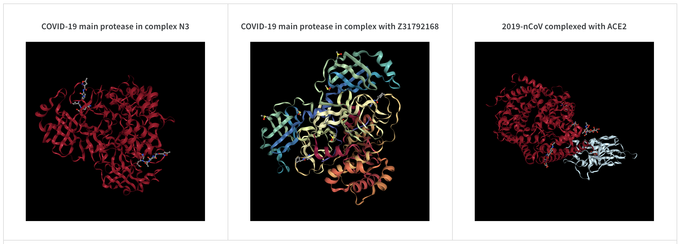
When your run finishes, you'll be able to interact with 3D visualizations of your molecules in the UI.
[See a live example using AlphaFold](https://wandb.me/alphafold-workspace)
### PNG image
[`wandb.Image`](/models/ref/python/data-types/image) converts `numpy` arrays or instances of `PILImage` to PNGs by default.
```python theme={null}
run.log({"example": wandb.Image(...)})
# Or multiple images
run.log({"example": [wandb.Image(...) for img in images]})
```
### Video
Videos are logged using the [`wandb.Video`](/models/ref/python/) data type:
```python theme={null}
run.log({"example": wandb.Video("myvideo.mp4")})
```
Now you can view videos in the media browser. Go to your project workspace, run workspace, or report and click **Add visualization** to add a rich media panel.
## 2D view of a molecule
You can log a 2D view of a molecule using the [`wandb.Image`](/models/ref/python/data-types/image) data type and [`rdkit`](https://www.rdkit.org/docs/index.html):
```python theme={null}
molecule = rdkit.Chem.MolFromSmiles("CC(=O)O")
rdkit.Chem.AllChem.Compute2DCoords(molecule)
rdkit.Chem.AllChem.GenerateDepictionMatching2DStructure(molecule, molecule)
pil_image = rdkit.Chem.Draw.MolToImage(molecule, size=(300, 300))
run.log({"acetic_acid": wandb.Image(pil_image)})
```
## Other media
W\&B also supports logging of a variety of other media types.
### Audio
```python theme={null}
run.log({"whale songs": wandb.Audio(np_array, caption="OooOoo", sample_rate=32)})
```
A maximum of 100 audio clips can be logged per step. For more usage information, see [`audio-file`](/models/ref/query-panel/audio-file).
### Video
```python theme={null}
run.log({"video": wandb.Video(numpy_array_or_path_to_video, fps=4, format="gif")})
```
If a numpy array is supplied we assume the dimensions are, in order: time, channels, width, height. By default we create a 4 fps gif image ([`ffmpeg`](https://www.ffmpeg.org) and the [`moviepy`](https://pypi.org/project/moviepy/) python library are required when passing numpy objects). Supported formats are `"gif"`, `"mp4"`, `"webm"`, and `"ogg"`. If you pass a string to `wandb.Video` we assert the file exists and is a supported format before uploading to wandb. Passing a `BytesIO` object will create a temporary file with the specified format as the extension.
On the W\&B [Run](/models/runs/) and [Project](/models/track/project-page/) Pages, you will see your videos in the Media section.
For more usage information, see [`video-file`](/models/ref/query-panel/video-file).
### Text
Use `wandb.Table` to log text in tables to show up in the UI. By default, the column headers are `["Input", "Output", "Expected"]`. To ensure optimal UI performance, the default maximum number of rows is set to 10,000. However, you can explicitly override the maximum with `wandb.Table.MAX_ROWS = {DESIRED_MAX}`.
```python theme={null}
with wandb.init(project="my_project") as run:
columns = ["Text", "Predicted Sentiment", "True Sentiment"]
# Method 1
data = [["I love my phone", "1", "1"], ["My phone sucks", "0", "-1"]]
table = wandb.Table(data=data, columns=columns)
run.log({"examples": table})
# Method 2
table = wandb.Table(columns=columns)
table.add_data("I love my phone", "1", "1")
table.add_data("My phone sucks", "0", "-1")
run.log({"examples": table})
```
You can also pass a pandas `DataFrame` object.
```python theme={null}
table = wandb.Table(dataframe=my_dataframe)
```
For more usage information, see [`string`](/models/ref/query-panel/).
### HTML
```python theme={null}
run.log({"custom_file": wandb.Html(open("some.html"))})
run.log({"custom_string": wandb.Html('Link')})
```
Log custom HTML at any key to expose an HTML panel on the run page. By default, we inject default styles; you can turn off default styles by passing `inject=False`.
```python theme={null}
run.log({"custom_file": wandb.Html(open("some.html"), inject=False)})
```
For more usage information, see [`html-file`](/models/ref/query-panel/html-file).
 Images can be logged directly from NumPy arrays, as PIL images, or from the filesystem.
Each time you log images from a step, they are available in the UI. Expand the image panel, then use the step slider to look at images from different steps. This makes it easy to compare how a model's output changes during training. Click a media panel to view an image in full-screen mode; there you can zoom and pan, including with [keyboard shortcuts](/models/app/keyboard-shortcuts#media-panels).
To compare images or videos from different runs, steps, or indices in one view, use [Compare mode](/models/app/features/panels/media#compare-mode) in a media panel.
Images can be logged directly from NumPy arrays, as PIL images, or from the filesystem.
Each time you log images from a step, they are available in the UI. Expand the image panel, then use the step slider to look at images from different steps. This makes it easy to compare how a model's output changes during training. Click a media panel to view an image in full-screen mode; there you can zoom and pan, including with [keyboard shortcuts](/models/app/keyboard-shortcuts#media-panels).
To compare images or videos from different runs, steps, or indices in one view, use [Compare mode](/models/app/features/panels/media#compare-mode) in a media panel.
 To log an overlay, provide a dictionary with the following keys and values to the `masks` keyword argument of `wandb.Image`:
* one of two keys representing the image mask:
* `"mask_data"`: a 2D NumPy array containing an integer class label for each pixel
* `"path"`: (string) a path to a saved image mask file
* `"class_labels"`: (optional) a dictionary mapping the integer class labels in the image mask to their readable class names
To log multiple masks, log a mask dictionary with multiple keys, as in the code snippet below.
[See a live example](https://app.wandb.ai/stacey/deep-drive/reports/Image-Masks-for-Semantic-Segmentation--Vmlldzo4MTUwMw)
[Sample code](https://colab.research.google.com/drive/1SOVl3EvW82Q4QKJXX6JtHye4wFix_P4J)
```python theme={null}
mask_data = np.array([[1, 2, 2, ..., 2, 2, 1], ...])
class_labels = {1: "tree", 2: "car", 3: "road"}
mask_img = wandb.Image(
image,
masks={
"predictions": {"mask_data": mask_data, "class_labels": class_labels},
"ground_truth": {
# ...
},
# ...
},
)
```
Segmentation masks for a key are defined at each step (each call to `run.log()`).
* If steps provide different values for the same mask key, only the most recent value for the key is applied to the image.
* If steps provide different mask keys, all values for each key are shown, but only those defined in the step being viewed are applied to the image. Toggling the visibility of masks not defined in the step do not change the image.
To log an overlay, provide a dictionary with the following keys and values to the `masks` keyword argument of `wandb.Image`:
* one of two keys representing the image mask:
* `"mask_data"`: a 2D NumPy array containing an integer class label for each pixel
* `"path"`: (string) a path to a saved image mask file
* `"class_labels"`: (optional) a dictionary mapping the integer class labels in the image mask to their readable class names
To log multiple masks, log a mask dictionary with multiple keys, as in the code snippet below.
[See a live example](https://app.wandb.ai/stacey/deep-drive/reports/Image-Masks-for-Semantic-Segmentation--Vmlldzo4MTUwMw)
[Sample code](https://colab.research.google.com/drive/1SOVl3EvW82Q4QKJXX6JtHye4wFix_P4J)
```python theme={null}
mask_data = np.array([[1, 2, 2, ..., 2, 2, 1], ...])
class_labels = {1: "tree", 2: "car", 3: "road"}
mask_img = wandb.Image(
image,
masks={
"predictions": {"mask_data": mask_data, "class_labels": class_labels},
"ground_truth": {
# ...
},
# ...
},
)
```
Segmentation masks for a key are defined at each step (each call to `run.log()`).
* If steps provide different values for the same mask key, only the most recent value for the key is applied to the image.
* If steps provide different mask keys, all values for each key are shown, but only those defined in the step being viewed are applied to the image. Toggling the visibility of masks not defined in the step do not change the image.
 [See a live example](https://app.wandb.ai/stacey/yolo-drive/reports/Bounding-Boxes-for-Object-Detection--Vmlldzo4Nzg4MQ)
To log a bounding box, you'll need to provide a dictionary with the following keys and values to the boxes keyword argument of `wandb.Image`:
* `box_data`: a list of dictionaries, one for each box. The box dictionary format is described below.
* `position`: a dictionary representing the position and size of the box in one of two formats, as described below. Boxes need not all use the same format.
* *Option 1:* `{"minX", "maxX", "minY", "maxY"}`. Provide a set of coordinates defining the upper and lower bounds of each box dimension.
* *Option 2:* `{"middle", "width", "height"}`. Provide a set of coordinates specifying the `middle` coordinates as `[x,y]`, and `width` and `height` as scalars.
* `class_id`: an integer representing the class identity of the box. See `class_labels` key below.
* `scores`: a dictionary of string labels and numeric values for scores. Can be used for filtering boxes in the UI.
* `domain`: specify the units/format of the box coordinates. **Set this to "pixel"** if the box coordinates are expressed in pixel space, such as integers within the bounds of the image dimensions. By default, the domain is assumed to be a fraction/percentage of the image, expressed as a floating point number between 0 and 1.
* `box_caption`: (optional) a string to be displayed as the label text on this box
* `class_labels`: (optional) A dictionary mapping `class_id`s to strings. By default we will generate class labels `class_0`, `class_1`, etc.
Check out this example:
```python theme={null}
import wandb
class_id_to_label = {
1: "car",
2: "road",
3: "building",
# ...
}
img = wandb.Image(
image,
boxes={
"predictions": {
"box_data": [
{
# one box expressed in the default relative/fractional domain
"position": {"minX": 0.1, "maxX": 0.2, "minY": 0.3, "maxY": 0.4},
"class_id": 2,
"box_caption": class_id_to_label[2],
"scores": {"acc": 0.1, "loss": 1.2},
# another box expressed in the pixel domain
# (for illustration purposes only, all boxes are likely
# to be in the same domain/format)
"position": {"middle": [150, 20], "width": 68, "height": 112},
"domain": "pixel",
"class_id": 3,
"box_caption": "a building",
"scores": {"acc": 0.5, "loss": 0.7},
# ...
# Log as many boxes an as needed
}
],
"class_labels": class_id_to_label,
},
# Log each meaningful group of boxes with a unique key name
"ground_truth": {
# ...
},
},
)
with wandb.init(project="my_project") as run:
run.log({"driving_scene": img})
```
[See a live example](https://app.wandb.ai/stacey/yolo-drive/reports/Bounding-Boxes-for-Object-Detection--Vmlldzo4Nzg4MQ)
To log a bounding box, you'll need to provide a dictionary with the following keys and values to the boxes keyword argument of `wandb.Image`:
* `box_data`: a list of dictionaries, one for each box. The box dictionary format is described below.
* `position`: a dictionary representing the position and size of the box in one of two formats, as described below. Boxes need not all use the same format.
* *Option 1:* `{"minX", "maxX", "minY", "maxY"}`. Provide a set of coordinates defining the upper and lower bounds of each box dimension.
* *Option 2:* `{"middle", "width", "height"}`. Provide a set of coordinates specifying the `middle` coordinates as `[x,y]`, and `width` and `height` as scalars.
* `class_id`: an integer representing the class identity of the box. See `class_labels` key below.
* `scores`: a dictionary of string labels and numeric values for scores. Can be used for filtering boxes in the UI.
* `domain`: specify the units/format of the box coordinates. **Set this to "pixel"** if the box coordinates are expressed in pixel space, such as integers within the bounds of the image dimensions. By default, the domain is assumed to be a fraction/percentage of the image, expressed as a floating point number between 0 and 1.
* `box_caption`: (optional) a string to be displayed as the label text on this box
* `class_labels`: (optional) A dictionary mapping `class_id`s to strings. By default we will generate class labels `class_0`, `class_1`, etc.
Check out this example:
```python theme={null}
import wandb
class_id_to_label = {
1: "car",
2: "road",
3: "building",
# ...
}
img = wandb.Image(
image,
boxes={
"predictions": {
"box_data": [
{
# one box expressed in the default relative/fractional domain
"position": {"minX": 0.1, "maxX": 0.2, "minY": 0.3, "maxY": 0.4},
"class_id": 2,
"box_caption": class_id_to_label[2],
"scores": {"acc": 0.1, "loss": 1.2},
# another box expressed in the pixel domain
# (for illustration purposes only, all boxes are likely
# to be in the same domain/format)
"position": {"middle": [150, 20], "width": 68, "height": 112},
"domain": "pixel",
"class_id": 3,
"box_caption": "a building",
"scores": {"acc": 0.5, "loss": 0.7},
# ...
# Log as many boxes an as needed
}
],
"class_labels": class_id_to_label,
},
# Log each meaningful group of boxes with a unique key name
"ground_truth": {
# ...
},
},
)
with wandb.init(project="my_project") as run:
run.log({"driving_scene": img})
```
 To log Segmentation Masks in tables, you will need to provide a `wandb.Image` object for each row in the table.
An example is provided in the Code snippet below:
```python theme={null}
table = wandb.Table(columns=["ID", "Image"])
for id, img, label in zip(ids, images, labels):
mask_img = wandb.Image(
img,
masks={
"prediction": {"mask_data": label, "class_labels": class_labels}
# ...
},
)
table.add_data(id, mask_img)
with wandb.init(project="my_project") as run:
run.log({"Table": table})
```
To log Segmentation Masks in tables, you will need to provide a `wandb.Image` object for each row in the table.
An example is provided in the Code snippet below:
```python theme={null}
table = wandb.Table(columns=["ID", "Image"])
for id, img, label in zip(ids, images, labels):
mask_img = wandb.Image(
img,
masks={
"prediction": {"mask_data": label, "class_labels": class_labels}
# ...
},
)
table.add_data(id, mask_img)
with wandb.init(project="my_project") as run:
run.log({"Table": table})
```
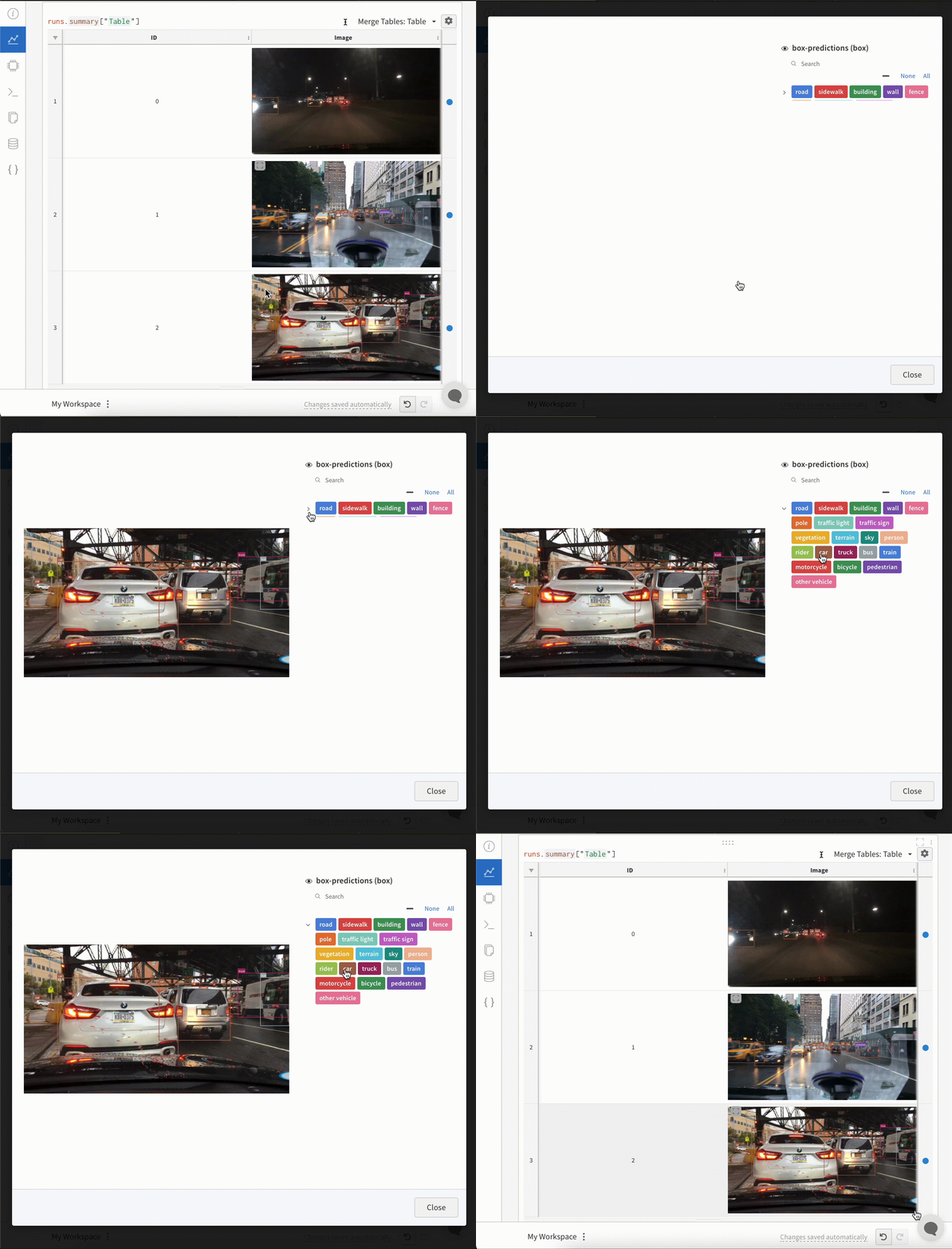 To log Images with Bounding Boxes in tables, you will need to provide a `wandb.Image` object for each row in the table.
An example is provided in the code snippet below:
```python theme={null}
table = wandb.Table(columns=["ID", "Image"])
for id, img, boxes in zip(ids, images, boxes_set):
box_img = wandb.Image(
img,
boxes={
"prediction": {
"box_data": [
{
"position": {
"minX": box["minX"],
"minY": box["minY"],
"maxX": box["maxX"],
"maxY": box["maxY"],
},
"class_id": box["class_id"],
"box_caption": box["caption"],
"domain": "pixel",
}
for box in boxes
],
"class_labels": class_labels,
}
},
)
```
To log Images with Bounding Boxes in tables, you will need to provide a `wandb.Image` object for each row in the table.
An example is provided in the code snippet below:
```python theme={null}
table = wandb.Table(columns=["ID", "Image"])
for id, img, boxes in zip(ids, images, boxes_set):
box_img = wandb.Image(
img,
boxes={
"prediction": {
"box_data": [
{
"position": {
"minX": box["minX"],
"minY": box["minY"],
"maxX": box["maxX"],
"maxY": box["maxY"],
},
"class_id": box["class_id"],
"box_caption": box["caption"],
"domain": "pixel",
}
for box in boxes
],
"class_labels": class_labels,
}
},
)
```
 ### PNG image
[`wandb.Image`](/models/ref/python/data-types/image) converts `numpy` arrays or instances of `PILImage` to PNGs by default.
```python theme={null}
run.log({"example": wandb.Image(...)})
# Or multiple images
run.log({"example": [wandb.Image(...) for img in images]})
```
### Video
Videos are logged using the [`wandb.Video`](/models/ref/python/) data type:
```python theme={null}
run.log({"example": wandb.Video("myvideo.mp4")})
```
Now you can view videos in the media browser. Go to your project workspace, run workspace, or report and click **Add visualization** to add a rich media panel.
## 2D view of a molecule
You can log a 2D view of a molecule using the [`wandb.Image`](/models/ref/python/data-types/image) data type and [`rdkit`](https://www.rdkit.org/docs/index.html):
```python theme={null}
molecule = rdkit.Chem.MolFromSmiles("CC(=O)O")
rdkit.Chem.AllChem.Compute2DCoords(molecule)
rdkit.Chem.AllChem.GenerateDepictionMatching2DStructure(molecule, molecule)
pil_image = rdkit.Chem.Draw.MolToImage(molecule, size=(300, 300))
run.log({"acetic_acid": wandb.Image(pil_image)})
```
## Other media
W\&B also supports logging of a variety of other media types.
### Audio
```python theme={null}
run.log({"whale songs": wandb.Audio(np_array, caption="OooOoo", sample_rate=32)})
```
A maximum of 100 audio clips can be logged per step. For more usage information, see [`audio-file`](/models/ref/query-panel/audio-file).
### Video
```python theme={null}
run.log({"video": wandb.Video(numpy_array_or_path_to_video, fps=4, format="gif")})
```
If a numpy array is supplied we assume the dimensions are, in order: time, channels, width, height. By default we create a 4 fps gif image ([`ffmpeg`](https://www.ffmpeg.org) and the [`moviepy`](https://pypi.org/project/moviepy/) python library are required when passing numpy objects). Supported formats are `"gif"`, `"mp4"`, `"webm"`, and `"ogg"`. If you pass a string to `wandb.Video` we assert the file exists and is a supported format before uploading to wandb. Passing a `BytesIO` object will create a temporary file with the specified format as the extension.
On the W\&B [Run](/models/runs/) and [Project](/models/track/project-page/) Pages, you will see your videos in the Media section.
For more usage information, see [`video-file`](/models/ref/query-panel/video-file).
### Text
Use `wandb.Table` to log text in tables to show up in the UI. By default, the column headers are `["Input", "Output", "Expected"]`. To ensure optimal UI performance, the default maximum number of rows is set to 10,000. However, you can explicitly override the maximum with `wandb.Table.MAX_ROWS = {DESIRED_MAX}`.
```python theme={null}
with wandb.init(project="my_project") as run:
columns = ["Text", "Predicted Sentiment", "True Sentiment"]
# Method 1
data = [["I love my phone", "1", "1"], ["My phone sucks", "0", "-1"]]
table = wandb.Table(data=data, columns=columns)
run.log({"examples": table})
# Method 2
table = wandb.Table(columns=columns)
table.add_data("I love my phone", "1", "1")
table.add_data("My phone sucks", "0", "-1")
run.log({"examples": table})
```
You can also pass a pandas `DataFrame` object.
```python theme={null}
table = wandb.Table(dataframe=my_dataframe)
```
For more usage information, see [`string`](/models/ref/query-panel/).
### HTML
```python theme={null}
run.log({"custom_file": wandb.Html(open("some.html"))})
run.log({"custom_string": wandb.Html('Link')})
```
Log custom HTML at any key to expose an HTML panel on the run page. By default, we inject default styles; you can turn off default styles by passing `inject=False`.
```python theme={null}
run.log({"custom_file": wandb.Html(open("some.html"), inject=False)})
```
For more usage information, see [`html-file`](/models/ref/query-panel/html-file).
### PNG image
[`wandb.Image`](/models/ref/python/data-types/image) converts `numpy` arrays or instances of `PILImage` to PNGs by default.
```python theme={null}
run.log({"example": wandb.Image(...)})
# Or multiple images
run.log({"example": [wandb.Image(...) for img in images]})
```
### Video
Videos are logged using the [`wandb.Video`](/models/ref/python/) data type:
```python theme={null}
run.log({"example": wandb.Video("myvideo.mp4")})
```
Now you can view videos in the media browser. Go to your project workspace, run workspace, or report and click **Add visualization** to add a rich media panel.
## 2D view of a molecule
You can log a 2D view of a molecule using the [`wandb.Image`](/models/ref/python/data-types/image) data type and [`rdkit`](https://www.rdkit.org/docs/index.html):
```python theme={null}
molecule = rdkit.Chem.MolFromSmiles("CC(=O)O")
rdkit.Chem.AllChem.Compute2DCoords(molecule)
rdkit.Chem.AllChem.GenerateDepictionMatching2DStructure(molecule, molecule)
pil_image = rdkit.Chem.Draw.MolToImage(molecule, size=(300, 300))
run.log({"acetic_acid": wandb.Image(pil_image)})
```
## Other media
W\&B also supports logging of a variety of other media types.
### Audio
```python theme={null}
run.log({"whale songs": wandb.Audio(np_array, caption="OooOoo", sample_rate=32)})
```
A maximum of 100 audio clips can be logged per step. For more usage information, see [`audio-file`](/models/ref/query-panel/audio-file).
### Video
```python theme={null}
run.log({"video": wandb.Video(numpy_array_or_path_to_video, fps=4, format="gif")})
```
If a numpy array is supplied we assume the dimensions are, in order: time, channels, width, height. By default we create a 4 fps gif image ([`ffmpeg`](https://www.ffmpeg.org) and the [`moviepy`](https://pypi.org/project/moviepy/) python library are required when passing numpy objects). Supported formats are `"gif"`, `"mp4"`, `"webm"`, and `"ogg"`. If you pass a string to `wandb.Video` we assert the file exists and is a supported format before uploading to wandb. Passing a `BytesIO` object will create a temporary file with the specified format as the extension.
On the W\&B [Run](/models/runs/) and [Project](/models/track/project-page/) Pages, you will see your videos in the Media section.
For more usage information, see [`video-file`](/models/ref/query-panel/video-file).
### Text
Use `wandb.Table` to log text in tables to show up in the UI. By default, the column headers are `["Input", "Output", "Expected"]`. To ensure optimal UI performance, the default maximum number of rows is set to 10,000. However, you can explicitly override the maximum with `wandb.Table.MAX_ROWS = {DESIRED_MAX}`.
```python theme={null}
with wandb.init(project="my_project") as run:
columns = ["Text", "Predicted Sentiment", "True Sentiment"]
# Method 1
data = [["I love my phone", "1", "1"], ["My phone sucks", "0", "-1"]]
table = wandb.Table(data=data, columns=columns)
run.log({"examples": table})
# Method 2
table = wandb.Table(columns=columns)
table.add_data("I love my phone", "1", "1")
table.add_data("My phone sucks", "0", "-1")
run.log({"examples": table})
```
You can also pass a pandas `DataFrame` object.
```python theme={null}
table = wandb.Table(dataframe=my_dataframe)
```
For more usage information, see [`string`](/models/ref/query-panel/).
### HTML
```python theme={null}
run.log({"custom_file": wandb.Html(open("some.html"))})
run.log({"custom_string": wandb.Html('Link')})
```
Log custom HTML at any key to expose an HTML panel on the run page. By default, we inject default styles; you can turn off default styles by passing `inject=False`.
```python theme={null}
run.log({"custom_file": wandb.Html(open("some.html"), inject=False)})
```
For more usage information, see [`html-file`](/models/ref/query-panel/html-file).