Try in Colab
アーティファクトについて
ギリシャのアンフォラのように、アーティファクトは生成されたオブジェクト、つまりプロセスの出力です。 MLでは、最も重要なアーティファクトは datasets と models です。 そして、コロナドの十字架のように、これらの重要なアーティファクトは博物館に保管されるべきです。 それは、あなたやあなたのチーム、そして広範な ML コミュニティがそれらから学べるように、カタログ化されて整理されるべきだということです。 結局のところ、トレーニングを追跡しない人々はそれを繰り返す運命にあります。 私たちの Artifacts API を使用することで、Artifact を W&B Run の出力としてログしたり、Run の入力として Artifact を使用したりできます。
この図では、トレーニング run がデータセットを取り込み、モデルを生成します。
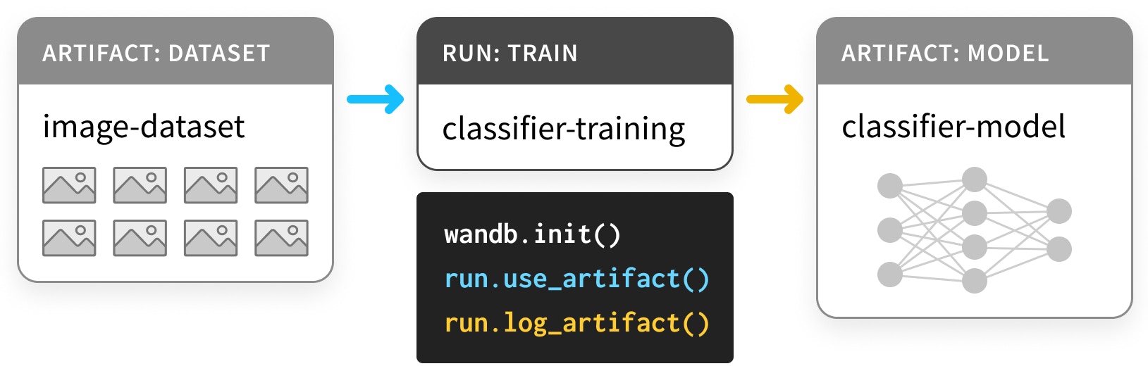
Artifact と Run は、Artifact と Run のノードを持ち、それを消費または生成する Run に接続する矢印を持つ、有向グラフ(二部 DAG)を形成します。
アーティファクトを使用してモデルとデータセットを追跡する
インストールとインポート
Artifacts は、バージョン0.9.2 以降の私たちの Python ライブラリの一部です。
ほとんどの ML Python スタックの部分と同様に、pip で利用可能です。
データセットをログする
まず、いくつかの Artifacts を定義しましょう。 この例は、PyTorch の “Basic MNIST Example” を基にしていますが、TensorFlow や他のフレームワーク、 あるいは純粋な Python でも同様に行うことができます。 データセットをtrain、validation、test として次のように定義します。
- パラメータを選択するための
trainセット - ハイパーパラメータを選択するための
validationセット - 最終モデルを評価するための
testセット
load するコードはデータを load_and_log するコードとは分かれています。
これは良い実践です。
これらのデータセットをアーティファクトとしてログするには、次の手順が必要です。
wandb.initでRunを作成する (L4)- データセットの
Artifactを作成する (L10) - 関連する
fileを保存してログする (L20, L23)
wandb.init
Artifact を生成する Run を作成するとき、その project に属することを明示する必要があります。
ワークフローに応じて、
プロジェクトは car-that-drives-itself のように大きいものであったり、
iterative-architecture-experiment-117 のように小さいものであったりします。
良い実践のルール: 可能であれば、同じ実行する様々な種類のジョブを追跡するために、Artifactを共有するすべてのRunを単一のプロジェクト内に保持してください。これによりシンプルになりますが、心配しないでください —Artifactはプロジェクト間で移動可能です。
Runs を作成する際に job_type を提供することをお勧めします。
これにより、Artifacts のグラフが整然とした状態を保つことができます。
良い実践のルール:job_typeは説明的であり、単一のパイプラインのステップに対応するものであるべきです。ここでは、preprocessデータとloadデータを分けて処理しています。
wandb.Artifact
何かを Artifact としてログするためには、最初に Artifact オブジェクトを作成する必要があります。
すべての Artifact には name があり — これが第一引数で設定されます。
良い実践のルール: name は説明的で、記憶しやすくタイプしやすいものであるべきです — 私たちは、コード内の変数名に対応するハイフンで区切られた名前を使用するのが好きです。
また、それには type があります。Run の job_type と同様に、これも Run と Artifact のグラフを整理するために使用されます。
良い実践のルール:また、辞書としてtypeはシンプルであるべきです。mnist-data-YYYYMMDDよりもdatasetやmodelのように。
description と metadata をアタッチすることもできます。
metadata は JSON にシリアライズ可能である必要があります。
良い実践のルール: metadata はできる限り詳しく記述するべきです。
artifact.new_file および run.log_artifact
一度 Artifact オブジェクトを作成したら、ファイルを追加する必要があります。
あなたはそれを正しく読みました。複数のファイル(s付き)です。
Artifact はディレクトリーのように構造化されており、
ファイルとサブディレクトリーを持っています。
良い実践のルール: 可能な限り、Artifact の内容を複数のファイルに分割してください。スケールする時が来たときに役立ちます。
new_file メソッドを使用して、ファイルを書き込むと同時にArtifact にアタッチします。
次のセクションでは、これらの2つの手順を分ける add_file メソッドを使用します。
すべてのファイルを追加したら、run.log_artifact を使用して wandb.ai にログする必要があります。
出力には Run ページの URL などのいくつかの URL が表示されることに気付くでしょう。
そこでは、ログされた Artifact を含む Run の結果を確認できます。
下記では、Run ページの他のコンポーネントをより活用する例をいくつか見ていきます。
ログされたデータセットアーティファクトを使用する
W&B 内のArtifact は博物館内のアーティファクトとは異なり、
単に保存されるだけでなく 使用 を想定しています。
それがどのように機能するか見てみましょう。
以下のセルでは、生のデータセットを取り込み、それを preprocess したデータセット(つまり normalize され正しい形に整形されたもの)を生成するパイプラインステップを定義しています。
また、コードの重要部分である preprocess を wandb とインターフェースするコードから分けています。
preprocess ステップを wandb.Artifact ログで装備するためのコードです。
以下の例では、use する Artifact が新たに登場し、log することは前のステップと同様です。
Artifact は、Run の入力と出力の両方です。
このステップが前のものとは異なる種類のジョブであることを明確にするために、新しい job_type、preprocess-data を使用します。
ステップ が preprocessed_data に metadata とともに保存されているということです。
実験を再現可能にしようとしている場合、多くのメタデータを収集することは良いアイデアです。
また、データセットは “large artifact” であるにもかかわらず、download ステップは1秒もかからずに完了します。
詳細は以下のマークダウンセルを展開してください。
run.use_artifact
これらのステップはよりシンプルです。消費者はその Artifact の name を知っていればいいだけです。その “bit more” とは、欲しい Artifact の特定のバージョンの alias です。
デフォルトでは、最後にアップロードされたバージョンが latest としてタグ付けされます。
それ以外の場合は v0 や v1 などで古いバージョンを選択することもでき、
また best や jit-script のような独自の alias を提供することもできます。
Docker Hub タグのように、alias は名前から : で分離されるため、私たちの求める Artifact は mnist-raw:latest になります。
良い実践のルール: alias を短く簡潔に保持します。 カスタムaliasであるlatestやbestのようなArtifactを使用して、ある条件を満たすものを指定します。
artifact.download
さて、あなたは download 呼び出しについて心配しているかもしれません。
別のコピーをダウンロードすると、メモリの負担が2倍になるのではないでしょうか?
心配しないでください。実際に何かをダウンロードする前に、
正しいバージョンがローカルにあるかどうか確認します。
これは torrenting や git を使用したバージョン管理 と同じ技術、ハッシュ化を使用しています。
Artifact が作成されログされると、
作業ディレクトリ内の artifacts というフォルダに
各 Artifact 用のサブディレクトリが埋まり始めます。
その内容を !tree artifacts で確認してください。
アーティファクトページ
Artifact をログし、使用したので、Run ページの Artifacts タブを見てみましょう。
wandb 出力からの Run ページの URL に移動し、
左サイドバーから “Artifacts” タブを選択します
(これはデータベースのアイコンで、
ホッケークラブを3つ重ねたようなものに見えるアイコンです)。
Input Artifacts テーブルや Output Artifacts テーブルのいずれかの行をクリックし、
その後に表示されるタブ (Overview, Metadata)
でログされた Artifact についての情報を確認してください。
私たちは特に Graph View を好んでいます。
デフォルトでは、Artifact の type と
Run の job_type を 2 つの種類のノードとして持ち、
消費と生成を表す矢印を持つグラフを表示します。
モデルをログする
これでArtifact API の動作がわかりましたが、
ML ワークフローを改善するために Artifact がどのように役立つかを理解するために、
パイプラインの終わりまでこの例を追ってみましょう。
ここでの最初のセルは、PyTorch で DNN model を構築します — 本当にシンプルな ConvNet です。
まず、model を初期化するだけで、トレーニングはしません。
そのため、すべての他の要素を一定に保ちながら複数のトレーニングを繰り返すことができます。
wandb.config オブジェクトを使用しています。
その dictionary バージョンの config object は本当に便利な metadata のピースなので、必ずそれを含めてください。
artifact.add_file
データセットのログ例のように、new_file を使用してファイルを書き込みアーティファクトに追加する代わりに、
ファイルを書き込んだ後に(ここでは torch.save により)それをアーティファクトに追加することもできます。
👍のルール: 重複を避けるために、できるだけ new_file を使用してください。
ログされたモデルアーティファクトを使用する
私たちがデータセットに対してuse_artifact を呼び出すことができたように、別の Run で initialized_model を使用することもできます。
この時は、model を train しましょう。
詳細については、
instrumenting W&B with PyTorch に関する Colab を参照してください。
Artifact を生成する Run を実行します。
最初の model ファイルを train する Run が終了し次第、
second は test_dataset 上の評価性能を evaluate することにより
trained-model Artifact を消費します。
また、ネットワークが最も混乱する32の例、
つまり categorical_crossentropy が最高の例を引き出します。
これは、データセットとモデルの問題を診断するための良い方法です。
Artifact 機能を追加することはないため、
コメントしません: これらは単に、
Artifact を use し、download し、
log しているだけです。