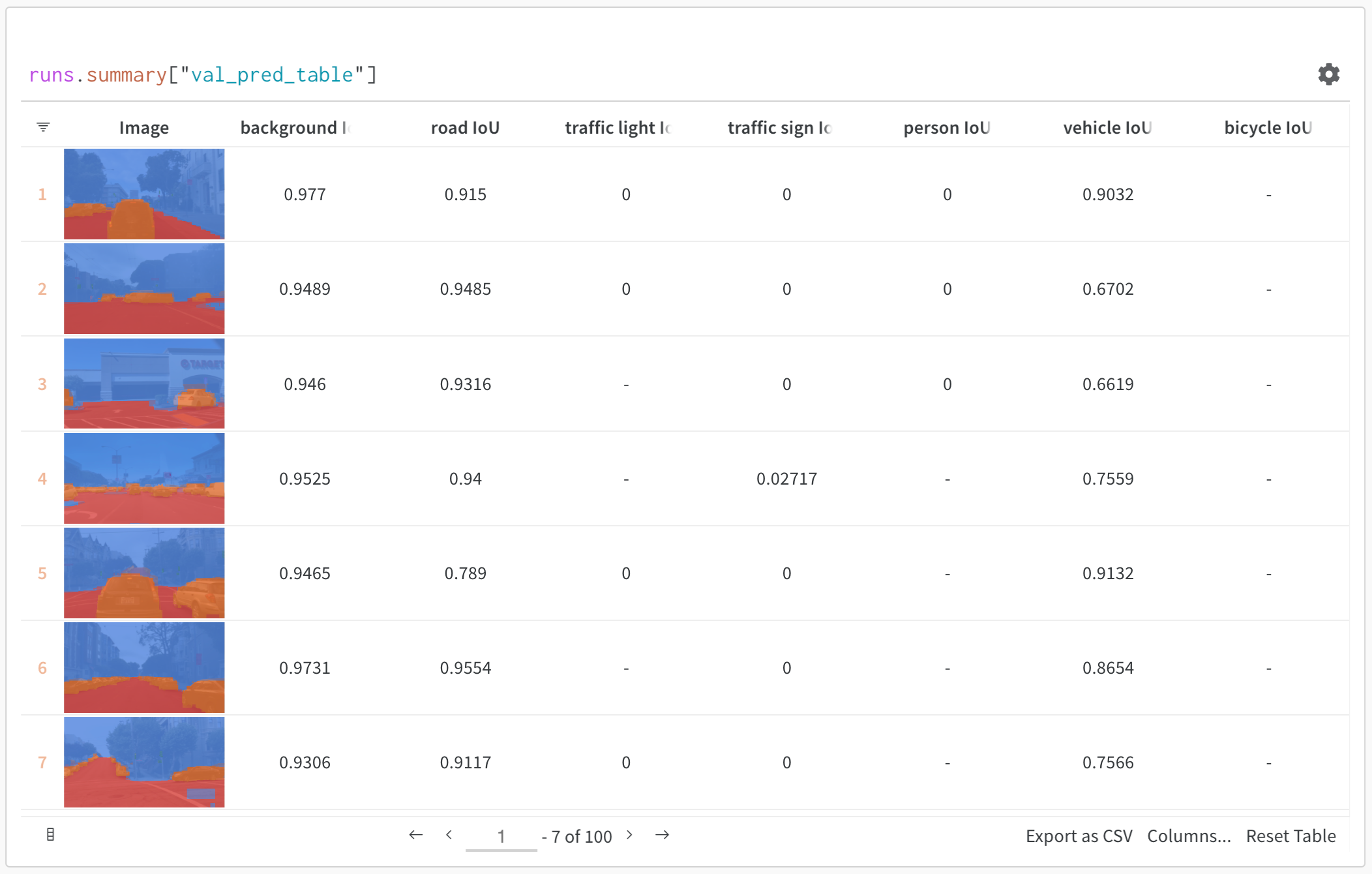
A Table is a two-dimensional grid of data where each column has a single type of data. Tables support primitive and numeric types, as well as nested lists, dictionaries, and rich media types.
import wandb
run = wandb.init(project="table-test")
# Create and log a new table.my_table = wandb.Table(columns=["a", "b"], data=[["a1", "b1"], ["a2", "b2"]])
run.log({"Table Name": my_table})
Pass a Pandas Dataframe to wandb.Table() to create a new table.
import wandb
import pandas as pd
df = pd.read_csv("my_data.csv")
run = wandb.init(project="df-table")
my_table = wandb.Table(dataframe=df)
wandb.log({"Table Name": my_table})
For more information on supported data types, see the wandb.Table in the W&B API Reference Guide.
2. Visualize tables in your project workspace
View the resulting table in your workspace.
Navigate to your project in the W&B App.
Select the name of your run in your project workspace. A new panel is added for each unique table key.
In this example, my_table, is logged under the key "Table Name".
3. Compare across model versions
Log sample tables from multiple W&B Runs and compare results in the project workspace. In this example workspace, we show how to combine rows from multiple different versions in the same table.
Use the table filter, sort, and grouping features to explore and evaluate model results.
2 - Log tables
Visualize and log tabular data with W&B Tables. A W&B Table is a two-dimensional grid of data where each column has a single type of data. Each row represents one or more data points logged to a W&B run. W&B Tables support primitive and numeric types, as well as nested lists, dictionaries, and rich media types.
W&B Tables are a specialized data type in W&B that are logged internally in W&B as artifacts objects.
You create and log table objects using the W&B Python SDK. When you create a table object, you specify the columns and data for the table and a mode. The mode determines how the table is logged and updated during your ML experiments.
Create and log a table
Initialize a new run with wandb.init().
Create a table object with the wandb.Table Class. Specify the columns and data for the table for the columns and data parameters, respectively. Though optional, it is recommended to set the log_mode parameter to one of the three modes: IMMUTABLE, MUTABLE, or INCREMENTAL. The default mode is IMMUTABLE. See Table Logging Modes in the next section for more information.
Log the table to W&B with run.log().
The following example shows how to create and log a table with two columns, a and b, and two rows of data, ["a1", "b1"] and ["a2", "b2"]:
import wandb
# Start a new runrun = wandb.init(project="table-demo")
# Create a table object with two columns and two rows of datamy_table = wandb.Table(
columns=["a", "b"],
data=[["a1", "b1"], ["a2", "b2"]],
log_mode="IMMUTABLE" )
# Log the table to W&Brun.log({"Table Name": my_table})
# Finish the runrun.finish()
Logging modes
The wandb.Tablelog_mode parameter determines how a table is logged and updated during your ML experiments. The log_mode parameter accepts one of three arguments: IMMUTABLE, MUTABLE, and INCREMENTAL. Each mode has different implications for how a table is logged, how it can be modified, and how it is rendered in the W&B App.
The following describes the three logging modes, the high-level differences, and common use case for each mode:
Mode
Definition
Use Cases
Benefits
IMMUTABLE
Once a table is logged to W&B, you cannot modify it.
- Storing tabular data generated at the end of a run for further analysis
- Minimal overhead when logged at the end of a run - All rows rendered in UI
MUTABLE
After you log a table to W&B, you can overwrite the existing table with a new one.
- Adding columns or rows to existing tables - Enriching results with new information
- Capture Table mutations - All rows rendered in UI
INCREMENTAL
Add batches of new rows to a table throughout the machine learning experiment.
- Adding rows to tables in batches - Long-running training jobs - Processing large datasets in batches - Monitoring ongoing results
- View updates on UI during training - Ability to step through increments
The next sections show example code snippets for each mode along with considerations when to use each mode.
MUTABLE mode
MUTABLE mode updates an existing table by replacing the existing table with a new one. MUTABLE mode is useful when you want to add new columns and rows to an existing table in a non iterative process. Within the UI, the table is rendered with all rows and columns, including the new ones added after the initial log.
In MUTABLE mode, the table object is replaced each time you log the table. Overwriting a table with a new one is computationally expensive and can be slow for large tables.
The following example shows how to create a table in MUTABLE mode, log it, and then add new columns to it. The table object is logged three times: once with the initial data, once with the confidence scores, and once with the final predictions.
The following example uses a placeholder function load_eval_data() to load data and a placeholder function model.predict() to make predictions. You will need to replace these with your own data loading and prediction functions.
import wandb
import numpy as np
run = wandb.init(project="mutable-table-demo")
# Create a table object with MUTABLE logging modetable = wandb.Table(columns=["input", "label", "prediction"],
log_mode="MUTABLE")
# Load data and make predictionsinputs, labels = load_eval_data() # Placeholder functionraw_preds = model.predict(inputs) # Placeholder functionfor inp, label, pred in zip(inputs, labels, raw_preds):
table.add_data(inp, label, pred)
# Step 1: Log initial data wandb.log({"eval_table": table}) # Log initial table# Step 2: Add confidence scores (e.g. max softmax)confidences = np.max(raw_preds, axis=1)
table.add_column("confidence", confidences)
run.log({"eval_table": table}) # Add confidence info# Step 3: Add post-processed predictions# (e.g., thresholded or smoothed outputs)post_preds = (confidences >0.7).astype(int)
table.add_column("final_prediction", post_preds)
wandb.log({"eval_table": table}) # Final update with another columnrun.finish()
If you only want to add new batches of rows (no columns) incrementally like in a training loop, consider using INCREMENTAL mode instead.
INCREMENTAL mode
In incremental mode, you log batches of rows to a table during the machine learning experiment. This is ideal for monitoring long-running jobs or when working with large tables that would be inefficient to log during the run for updates. Within the UI, the table is updated with new rows as they are logged, allowing you to view the latest data without having to wait for the entire run to finish. You can also step through the increments to view the table at different points in time.
Run workspaces in the W&B App have a limit of 100 increments. If you log more than 100 increments, only the most recent 100 are shown in the run workspace.
The following example creates a table in INCREMENTAL mode, logs it, and then adds new rows to it. Note that the table is logged once per training step (step).
The following example uses a placeholder function get_training_batch() to load data, a placeholder function train_model_on_batch() to train the model, and a placeholder function predict_on_batch() to make predictions. You will need to replace these with your own data loading, training, and prediction functions.
import wandb
run = wandb.init(project="incremental-table-demo")
# Create a table with INCREMENTAL logging modetable = wandb.Table(columns=["step", "input", "label", "prediction"],
log_mode="INCREMENTAL")
# Training loopfor step in range(get_num_batches()): # Placeholder function# Load batch data inputs, labels = get_training_batch(step) # Placeholder function# Train and predict train_model_on_batch(inputs, labels) # Placeholder function predictions = predict_on_batch(inputs) # Placeholder function# Add batch data to tablefor input_item, label, prediction in zip(inputs, labels, predictions):
table.add_data(step, input_item, label, prediction)
# Log the table incrementally wandb.log({"training_table": table}, step=step)
run.finish()
Incremental logging is generally more computationally efficient than logging a new table each time (log_mode=MUTABLE). However, the W&B App may not render all rows in the table if you log a large number of increments. If your goal is to update and view your table data while your run is ongoing and to have all the data available for analysis, consider using two tables. One with INCREMENTAL log mode and one with IMMUTABLE log mode.
The following example shows how to combine INCREMENTAL and IMMUTABLE logging modes to achieve this.
import wandb
run = wandb.init(project="combined-logging-example")
# Create an incremental table for efficient updates during trainingincr_table = wandb.Table(columns=["step", "input", "prediction", "label"],
log_mode="INCREMENTAL")
# Training loopfor step in range(get_num_batches()):
# Process batch inputs, labels = get_training_batch(step)
predictions = model.predict(inputs)
# Add data to incremental tablefor inp, pred, label in zip(inputs, predictions, labels):
incr_table.add_data(step, inp, pred, label)
# Log the incremental update (suffix with -incr to distinguish from final table) run.log({"table-incr": incr_table}, step=step)
# At the end of training, create a complete immutable table with all data# Using the default IMMUTABLE mode to preserve the complete datasetfinal_table = wandb.Table(columns=incr_table.columns, data=incr_table.data, log_mode="IMMUTABLE")
run.log({"table": final_table})
run.finish()
In this example, the incr_table is logged incrementally (with log_mode="INCREMENTAL") during training. This allows you to log and view updates to the table as new data is processed. At the end of training, an immutable table (final_table) is created with all data from the incremental table. The immutable table is logged to preserve the complete dataset for further analysis and it enables you to view all rows in the W&B App.
You can continue logging to an incremental table when resuming a run:
# Start or resume a runresumed_run = wandb.init(project="resume-incremental", id="your-run-id", resume="must")
# Create the incremental table; no need to populate with data from preivously logged table# Increments will be continue to be added to the Table artifact.table = wandb.Table(columns=["step", "metric"], log_mode="INCREMENTAL")
# Continue loggingfor step in range(resume_step, final_step):
metric = compute_metric(step)
table.add_data(step, metric)
resumed_run.log({"metrics": table}, step=step)
resumed_run.finish()
Increments are logged to a new table if you turn off summaries on a key used for the incremental table using wandb.define_metric("<table_key>", summary="none") or wandb.define_metric("*", summary="none").
Training with INCREMENTAL batch training
run = wandb.init(project="batch-training-incremental")
# Create an incremental tabletable = wandb.Table(columns=["step", "input", "label", "prediction"], log_mode="INCREMENTAL")
# Simulated training loopfor step in range(get_num_batches()):
# Load batch data inputs, labels = get_training_batch(step)
# Train the model on this batch train_model_on_batch(inputs, labels)
# Run model inference predictions = predict_on_batch(inputs)
# Add data to the tablefor input_item, label, prediction in zip(inputs, labels, predictions):
table.add_data(step, input_item, label, prediction)
# Log the current state of the table incrementally run.log({"training_table": table}, step=step)
run.finish()
3 - Visualize and analyze tables
Visualize and analyze W&B Tables.
Customize your W&B Tables to answer questions about your machine learning model’s performance, analyze your data, and more.
Interactively explore your data to:
Compare changes precisely across models, epochs, or individual examples
Understand higher-level patterns in your data
Capture and communicate your insights with visual samples
W&B Tables posses the following behaviors:
Stateless in an artifact context: any table logged alongside an artifact version resets to its default state after you close the browser window
Stateful in a workspace or report context: any changes you make to a table in a single run workspace, multi-run project workspace, or Report persists.
For information on how to save your current W&B Table view, see Save your view.
Compare two tables
Compare two tables with a merged view or a side-by-side view. For example, the image below demonstrates a table comparison of MNIST data.
Follow these steps to compare two tables:
Go to your project in the W&B App.
Select the artifacts icon on the left panel.
Select an artifact version.
In the following image we demonstrate a model’s predictions on MNIST validation data after each of five epochs (view interactive example here).
Hover over the second artifact version you want to compare in the sidebar and click Compare when it appears. For example, in the image below we select a version labeled as “v4” to compare to MNIST predictions made by the same model after 5 epochs of training.
Merged view
Initially you see both tables merged together. The first table selected has index 0 and a blue highlight, and the second table has index 1 and a yellow highlight. View a live example of merged tables here.
From the merged view, you can
choose the join key: use the dropdown at the top left to set the column to use as the join key for the two tables. Typically this is the unique identifier of each row, such as the filename of a specific example in your dataset or an incrementing index on your generated samples. Note that it’s currently possible to select any column, which may yield illegible tables and slow queries.
concatenate instead of join: select “concatenating all tables” in this dropdown to union all the rows from both tables into one larger Table instead of joining across their columns
reference each Table explicitly: use 0, 1, and * in the filter expression to explicitly specify a column in one or both table instances
visualize detailed numerical differences as histograms: compare the values in any cell at a glance
Side-by-side view
To view the two tables side-by-side, change the first dropdown from “Merge Tables: Table” to “List of: Table” and then update the “Page size” respectively. Here the first Table selected is on the left and the second one is on the right. Also, you can compare these tables vertically as well by clicking on the “Vertical” checkbox.
compare the tables at a glance: apply any operations (sort, filter, group) to both tables in tandem and spot any changes or differences quickly. For example, view the incorrect predictions grouped by guess, the hardest negatives overall, the confidence score distribution by true label, etc.
explore two tables independently: scroll through and focus on the side/rows of interest
Visualize how values change throughout your runs
View how values you log to a table change throughout your runs with a step slider. Slide the step slider to view the values logged at different steps. For example, you can view how the loss, accuracy, or other metrics change after each run.
he slider uses a key to determine the step value. The default key for the slider is _step, a special key that W&B automatically logs for you. The _step key is an integer that increments by 1 each time you call wandb.log() in your code.
To add a step slider to a W&B Table:
Navigate to your project’s workspace.
Click Add panel in the top right corner of the workspace.
Select Query panel.
Within the query expression editor, select runs and press Enter on your keyboard.
Click the gear icon to view the settings for the panel.
The following image shows a query panel with three W&B runs and the values they logged at step 295.
Within the W&B App UI you may notice duplicate values for multiple steps. This duplication can occur if multiple runs log the same value at different steps, or if a run does not log values at every step. If a value is missing for a given step, W&B uses the last value that was logged as the slider key.
Custom step key
The step key can be any numeric metric that you log in your runs as the step key, such as epoch or global_step. When you use a custom step key, W&B maps each value of that key to a step (_step) in the run.
This table shows how a custom step key epoch maps to _step values for three different runs: serene-sponge, lively-frog, and vague-cloud. Each row represents a call to wandb.log() at a particular _step in a run. The columns show the corresponding epoch values, if any, that were logged at those steps. Some _step values are omitted to save space.
The first time wandb.log was called, none of the runs logged an epoch value, so the table shows empty values for epoch.
_step
vague-cloud (epoch)
lively-frog(epoch)
serene-sponge (epoch)
1
2
1
4
1
2
5
1
6
3
8
2
4
10
5
12
3
6
14
7
15
2
16
4
8
18
9
20
3
5
10
Now, if the slider is set to epoch = 1, the following happens:
vague-cloud finds epoch = 1 and returns the value logged at _step = 5
lively-frog finds epoch = 1 and returns the value logged at _step = 4
serene-sponge finds epoch = 1 and returns the value logged at _step = 2
If the slider is set to epoch = 9:
vague-cloud also doesn’t log epoch = 9, so W&B uses the latest prior value epoch = 3 and returns the value logged at _step = 20
lively-frog doesn’t log epoch = 9, but the latest prior value is epoch = 5 so it returns the value logged at _step = 20
serene-sponge finds epoch = 9 and return the value logged at _step = 18
Log a table in an artifact for each meaningful step of training to analyze model performance over training time. For example, you could log a table at the end of every validation step, after every 50 epochs of training, or any frequency that makes sense for your pipeline. Use the side-by-side view to visualize changes in model predictions.
For a more detailed walkthrough of visualizing predictions across training time, see this report and this interactive notebook example.
Compare tables across model variants
Compare two artifact versions logged at the same step for two different models to analyze model performance across different configurations (hyperparameters, base architectures, and so forth).
For example, compare predictions between a baseline and a new model variant, 2x_layers_2x_lr, where the first convolutional layer doubles from 32 to 64, the second from 128 to 256, and the learning rate from 0.001 to 0.002. From this live example, use the side-by-side view and filter down to the incorrect predictions after 1 (left tab) versus 5 training epochs (right tab).
Save your view
Tables you interact with in the run workspace, project workspace, or a report automatically saves their view state. If you apply any table operations then close your browser, the table retains the last viewed configuration when you next navigate to the table.
Tables you interact with in the artifact context remains stateless.
To save a table from a workspace in a particular state, export it to a W&B Report. To export a table to report:
Select the kebab icon (three vertical dots) in the top right corner of your workspace visualization panel.
Select either Share panel or Add to report.
Examples
These reports highlight the different use cases of W&B Tables:
The following sections highlight some of the ways you can use tables:
View your data
Log metrics and rich media during model training or evaluation, then visualize results in a persistent database synced to the cloud, or to your hosting instance.
View, sort, filter, group, join, and query tables to understand your data and model performance—no need to browse static files or rerun analysis scripts.
Zoom in to visualize a specific prediction at a specific step. Zoom out to see the aggregate statistics, identify patterns of errors, and understand opportunities for improvement. This tool works for comparing steps from a single model training, or results across different model versions.
Interact with audio tables in this report on timbre transfer. You can compare a recorded whale song with a synthesized rendition of the same melody on an instrument like violin or trumpet. You can also record your own songs and explore their synthesized versions in W&B with this colab.
Text
Browse text samples from training data or generated output, dynamically group by relevant fields, and align your evaluation across model variants or experiment settings. Render text as Markdown or use visual diff mode to compare texts. Explore a simple character-based RNN for generating Shakespeare in this report.
Video
Browse and aggregate over videos logged during training to understand your models. Here is an early example using the SafeLife benchmark for RL agents seeking to minimize side effects
Like all W&B Artifacts, Tables can be converted into pandas dataframes for easy data exporting.
Convert table to artifact
First, you’ll need to convert the table to an artifact. The easiest way to do this using artifact.get(table, "table_name"):
# Create and log a new table.with wandb.init() as r:
artifact = wandb.Artifact("my_dataset", type="dataset")
table = wandb.Table(
columns=["a", "b", "c"], data=[(i, i *2, 2**i) for i in range(10)]
)
artifact.add(table, "my_table")
wandb.log_artifact(artifact)
# Retrieve the created table using the artifact you created.with wandb.init() as r:
artifact = r.use_artifact("my_dataset:latest")
table = artifact.get("my_table")
Convert artifact to Dataframe
Then, convert the table into a dataframe:
# Following from the last code example:df = table.get_dataframe()
Export Data
Now you can export using any method dataframe supports:
# Converting the table data to .csvdf.to_csv("example.csv", encoding="utf-8")