This is the multi-page printable view of this section. Click here to print.

Return to the regular view of this page.

Tables

Iterate on datasets and understand model predictions

Use W&B Tables to visualize and query tabular data. For example:

  • Compare how different models perform on the same test set
  • Identify patterns in your data
  • Look at sample model predictions visually
  • Query to find commonly misclassified examples
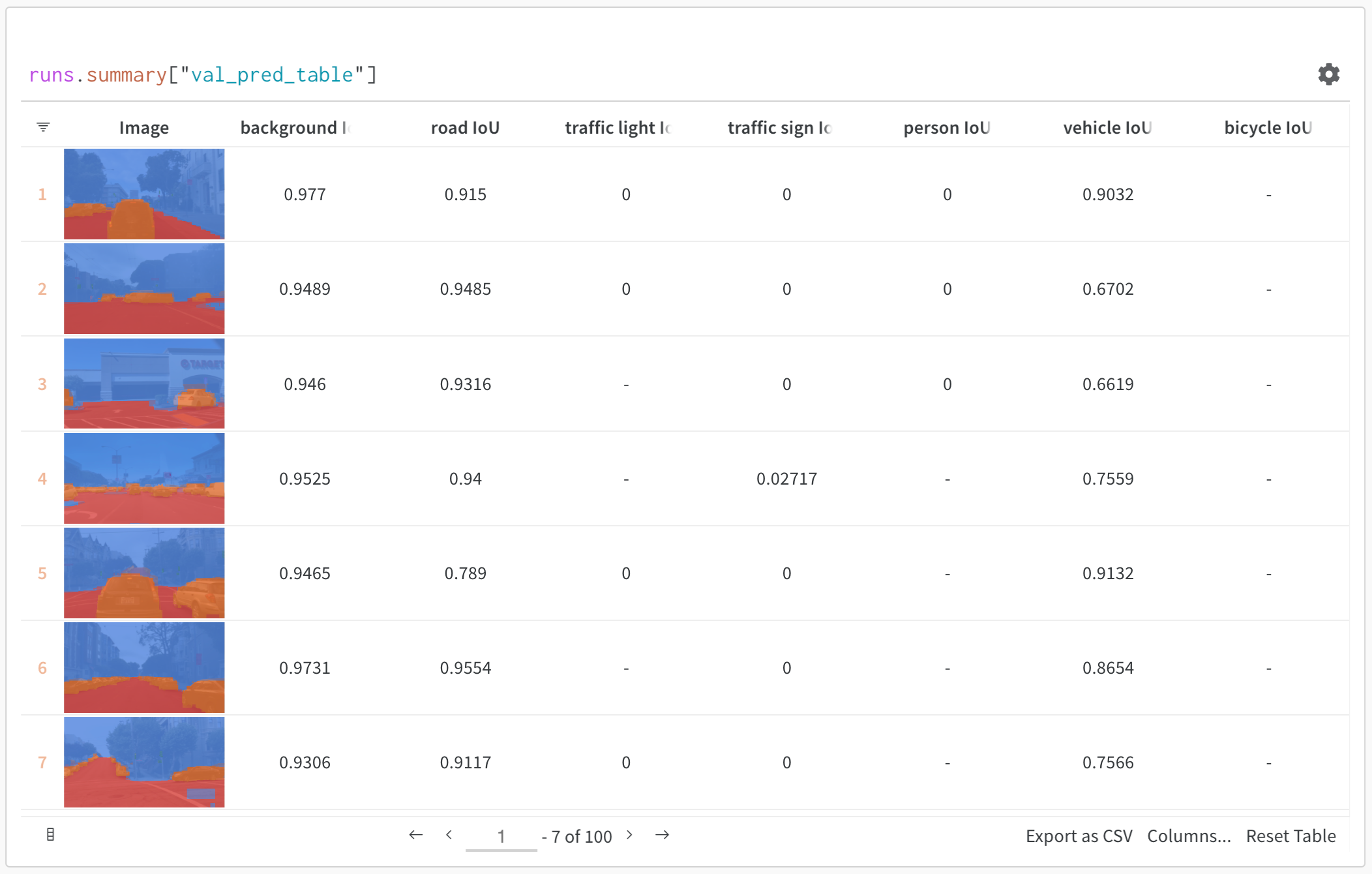
The above image shows a table with semantic segmentation and custom metrics. View this table here in this sample project from the W&B ML Course.

How it works

A Table is a two-dimensional grid of data where each column has a single type of data. Tables support primitive and numeric types, as well as nested lists, dictionaries, and rich media types.

Log a Table

Log a table with a few lines of code:

  • wandb.init(): Create a run to track results.
  • wandb.Table(): Create a new table object.
    • columns: Set the column names.
    • data: Set the contents of the table.
  • run.log(): Log the table to save it to W&B.
import wandb

run = wandb.init(project="table-test")
my_table = wandb.Table(columns=["a", "b"], data=[["a1", "b1"], ["a2", "b2"]])
run.log({"Table Name": my_table})

How to get started

  • Quickstart: Learn to log data tables, visualize data, and query data.
  • Tables Gallery: See example use cases for Tables.

1 - Tutorial: Log tables, visualize and query data

Explore how to use W&B Tables with this 5 minute Quickstart.

The following Quickstart demonstrates how to log data tables, visualize data, and query data.

Select the button below to try a PyTorch Quickstart example project on MNIST data.

1. Log a table

Log a table with W&B. You can either construct a new table or pass a Pandas Dataframe.

To construct and log a new Table, you will use:

  • wandb.init(): Create a run to track results.
  • wandb.Table(): Create a new table object.
    • columns: Set the column names.
    • data: Set the contents of each row.
  • run.log(): Log the table to save it to W&B.

Here’s an example:

import wandb

run = wandb.init(project="table-test")
# Create and log a new table.
my_table = wandb.Table(columns=["a", "b"], data=[["a1", "b1"], ["a2", "b2"]])
run.log({"Table Name": my_table})

Pass a Pandas Dataframe to wandb.Table() to create a new table.

import wandb
import pandas as pd

df = pd.read_csv("my_data.csv")

run = wandb.init(project="df-table")
my_table = wandb.Table(dataframe=df)
wandb.log({"Table Name": my_table})

For more information on supported data types, see the wandb.Table in the W&B API Reference Guide.

2. Visualize tables in your project workspace

View the resulting table in your workspace.

  1. Navigate to your project in the W&B App.
  2. Select the name of your run in your project workspace. A new panel is added for each unique table key.

In this example, my_table, is logged under the key "Table Name".

3. Compare across model versions

Log sample tables from multiple W&B Runs and compare results in the project workspace. In this example workspace, we show how to combine rows from multiple different versions in the same table.

Use the table filter, sort, and grouping features to explore and evaluate model results.

2 - Visualize and analyze tables

Visualize and analyze W&B Tables.

Customize your W&B Tables to answer questions about your machine learning model’s performance, analyze your data, and more.

Interactively explore your data to:

  • Compare changes precisely across models, epochs, or individual examples
  • Understand higher-level patterns in your data
  • Capture and communicate your insights with visual samples

How to view two tables

Compare two tables with a merged view or a side-by-side view. For example, the image below demonstrates a table comparison of MNIST data.

Left: mistakes after 1 training epochs, Right: mistakes after 5 epochs

Follow these steps to compare two tables:

  1. Go to your project in the W&B App.
  2. Select the artifacts icon on the left panel.
  3. Select an artifact version.

In the following image we demonstrate a model’s predictions on MNIST validation data after each of five epochs (view interactive example here).

Click on 'predictions' to view the Table
  1. Hover over the second artifact version you want to compare in the sidebar and click Compare when it appears. For example, in the image below we select a version labeled as “v4” to compare to MNIST predictions made by the same model after 5 epochs of training.
Preparing to compare model predictions after training for 1 epoch (v0, shown here) vs 5 epochs (v4)

Merged view

Initially you see both tables merged together. The first table selected has index 0 and a blue highlight, and the second table has index 1 and a yellow highlight. View a live example of merged tables here.

In the merged view, numerical columns appears as histograms by default

From the merged view, you can

  • choose the join key: use the dropdown at the top left to set the column to use as the join key for the two tables. Typically this is the unique identifier of each row, such as the filename of a specific example in your dataset or an incrementing index on your generated samples. Note that it’s currently possible to select any column, which may yield illegible tables and slow queries.
  • concatenate instead of join: select “concatenating all tables” in this dropdown to union all the rows from both tables into one larger Table instead of joining across their columns
  • reference each Table explicitly: use 0, 1, and * in the filter expression to explicitly specify a column in one or both table instances
  • visualize detailed numerical differences as histograms: compare the values in any cell at a glance

Side-by-side view

To view the two tables side-by-side, change the first dropdown from “Merge Tables: Table” to “List of: Table” and then update the “Page size” respectively. Here the first Table selected is on the left and the second one is on the right. Also, you can compare these tables vertically as well by clicking on the “Vertical” checkbox.

In the side-by-side view, Table rows are independent of each other.
  • compare the tables at a glance: apply any operations (sort, filter, group) to both tables in tandem and spot any changes or differences quickly. For example, view the incorrect predictions grouped by guess, the hardest negatives overall, the confidence score distribution by true label, etc.
  • explore two tables independently: scroll through and focus on the side/rows of interest

Compare artifacts

You can also compare tables across time or model variants.

Compare tables across time

Log a table in an artifact for each meaningful step of training to analyze model performance over training time. For example, you could log a table at the end of every validation step, after every 50 epochs of training, or any frequency that makes sense for your pipeline. Use the side-by-side view to visualize changes in model predictions.

For each label, the model makes fewer mistakes after 5 training epochs (R) than after 1 (L)

For a more detailed walkthrough of visualizing predictions across training time, see this report and this interactive notebook example.

Compare tables across model variants

Compare two artifact versions logged at the same step for two different models to analyze model performance across different configurations (hyperparameters, base architectures, and so forth).

For example, compare predictions between a baseline and a new model variant, 2x_layers_2x_lr, where the first convolutional layer doubles from 32 to 64, the second from 128 to 256, and the learning rate from 0.001 to 0.002. From this live example, use the side-by-side view and filter down to the incorrect predictions after 1 (left tab) versus 5 training epochs (right tab).

After 1 epoch, performance is mixed: precision improves for some classes and worsens for others.
After 5 epochs, the 'double' variant is catching up to the baseline.

Save your view

Tables you interact with in the run workspace, project workspace, or a report automatically saves their view state. If you apply any table operations then close your browser, the table retains the last viewed configuration when you next navigate to the table.

To save a table from a workspace in a particular state, export it to a W&B Report. To export a table to report:

  1. Select the kebob icon (three vertical dots) in the top right corner of your workspace visualization panel.
  2. Select either Share panel or Add to report.
Share panel creates a new report, Add to report lets you append to an existing report.

Examples

These reports highlight the different use cases of W&B Tables:

3 - Example tables

Examples of W&B Tables

The following sections highlight some of the ways you can use tables:

View your data

Log metrics and rich media during model training or evaluation, then visualize results in a persistent database synced to the cloud, or to your hosting instance.

Browse examples and verify the counts and distribution of your data

For example, check out this table that shows a balanced split of a photos dataset.

Interactively explore your data

View, sort, filter, group, join, and query tables to understand your data and model performance—no need to browse static files or rerun analysis scripts.

Listen to original songs and their synthesized versions (with timbre transfer)

For example, see this report on style-transferred audio.

Compare model versions

Quickly compare results across different training epochs, datasets, hyperparameter choices, model architectures etc.

See granular differences: the left model detects some red sidewalk, the right does not.

For example, see this table that compares two models on the same test images.

Track every detail and see the bigger picture

Zoom in to visualize a specific prediction at a specific step. Zoom out to see the aggregate statistics, identify patterns of errors, and understand opportunities for improvement. This tool works for comparing steps from a single model training, or results across different model versions.

For example, see this example table that analyzes results after one and then after five epochs on the MNIST dataset.

Example Projects with W&B Tables

The following highlight some real W&B Projects that use W&B Tables.

Image classification

Read this report, follow this colab, or explore this artifacts context to see how a CNN identifies ten types of living things (plants, bird, insects, etc) from iNaturalist photos.

Compare the distribution of true labels across two different models' predictions.

Audio

Interact with audio tables in this report on timbre transfer. You can compare a recorded whale song with a synthesized rendition of the same melody on an instrument like violin or trumpet. You can also record your own songs and explore their synthesized versions in W&B with this colab.

Text

Browse text samples from training data or generated output, dynamically group by relevant fields, and align your evaluation across model variants or experiment settings. Render text as Markdown or use visual diff mode to compare texts. Explore a simple character-based RNN for generating Shakespeare in this report.

Doubling the size of the hidden layer yields some more creative prompt completions.

Video

Browse and aggregate over videos logged during training to understand your models. Here is an early example using the SafeLife benchmark for RL agents seeking to minimize side effects

Browse easily through the few successful agents

Tabular data

View a report on how to split and pre-process tabular data with version control and de-duplication.

Tables and Artifacts work together to version control, label, and de-duplicate your dataset iterations

Comparing model variants (semantic segmentation)

An interactive notebook and live example of logging Tables for semantic segmentation and comparing different models. Try your own queries in this Table.

Find the best predictions across two models on the same test set

Analyzing improvement over training time

A detailed report on how to visualize predictions over time and the accompanying interactive notebook.

4 - Export table data

How to export data from tables.

Like all W&B Artifacts, Tables can be converted into pandas dataframes for easy data exporting.

Convert table to artifact

First, you’ll need to convert the table to an artifact. The easiest way to do this using artifact.get(table, "table_name"):

# Create and log a new table.
with wandb.init() as r:
    artifact = wandb.Artifact("my_dataset", type="dataset")
    table = wandb.Table(
        columns=["a", "b", "c"], data=[(i, i * 2, 2**i) for i in range(10)]
    )
    artifact.add(table, "my_table")
    wandb.log_artifact(artifact)

# Retrieve the created table using the artifact you created.
with wandb.init() as r:
    artifact = r.use_artifact("my_dataset:latest")
    table = artifact.get("my_table")

Convert artifact to Dataframe

Then, convert the table into a dataframe:

# Following from the last code example:
df = table.get_dataframe()

Export Data

Now you can export using any method dataframe supports:

# Converting the table data to .csv
df.to_csv("example.csv", encoding="utf-8")

Next Steps