Embed objects
4 minute read
Embeddings are used to represent objects (people, images, posts, words, etc…) with a list of numbers - sometimes referred to as a vector. In machine learning and data science use cases, embeddings can be generated using a variety of approaches across a range of applications. This page assumes the reader is familiar with embeddings and is interested in visually analyzing them inside of W&B.
Embedding Examples
Hello World
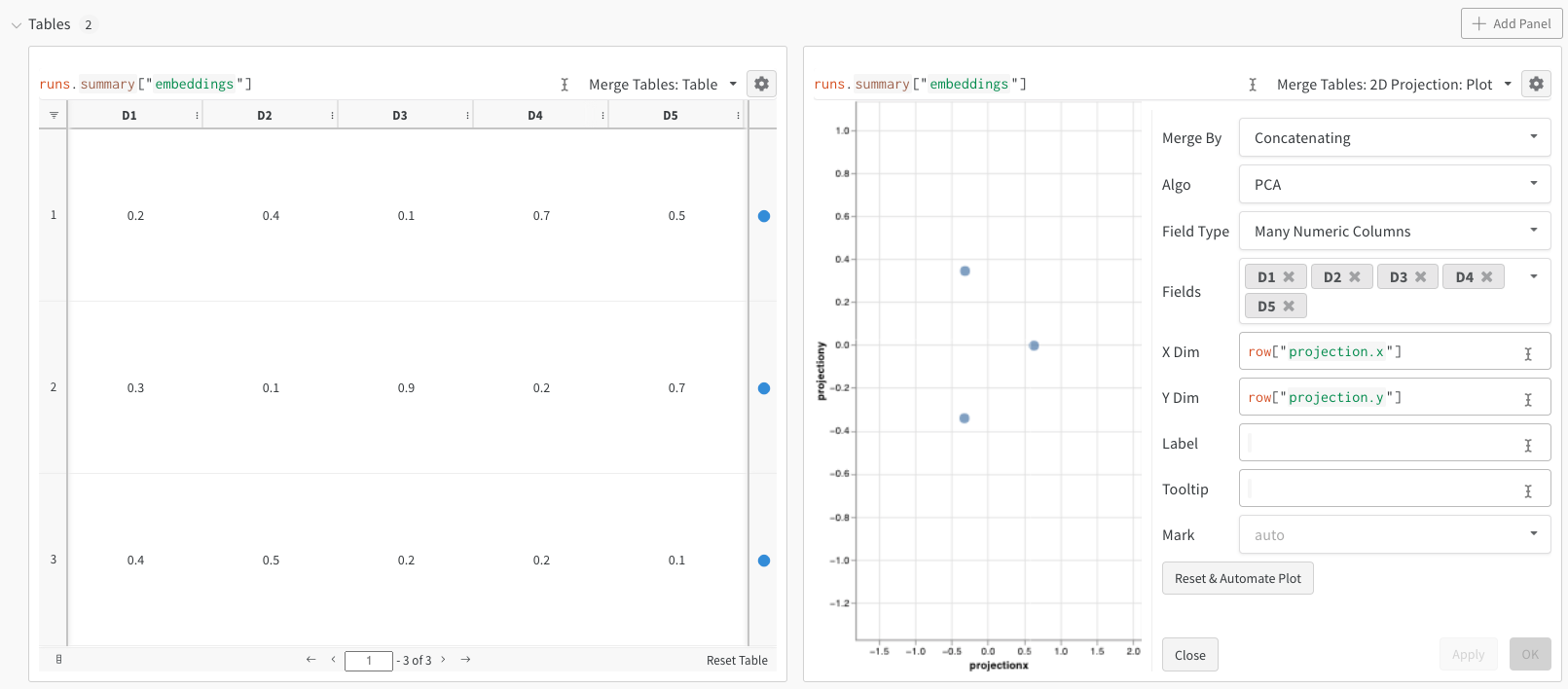
W&B allows you to log embeddings using the wandb.Table class. Consider the following example of 3 embeddings, each consisting of 5 dimensions:
After running the above code, the W&B dashboard will have a new Table containing your data. You can select 2D Projection from the upper right panel selector to plot the embeddings in 2 dimensions. Smart default will be automatically selected, which can be easily overridden in the configuration menu accessed by clicking the gear icon. In this example, we automatically use all 5 available numeric dimensions.
Digits MNIST
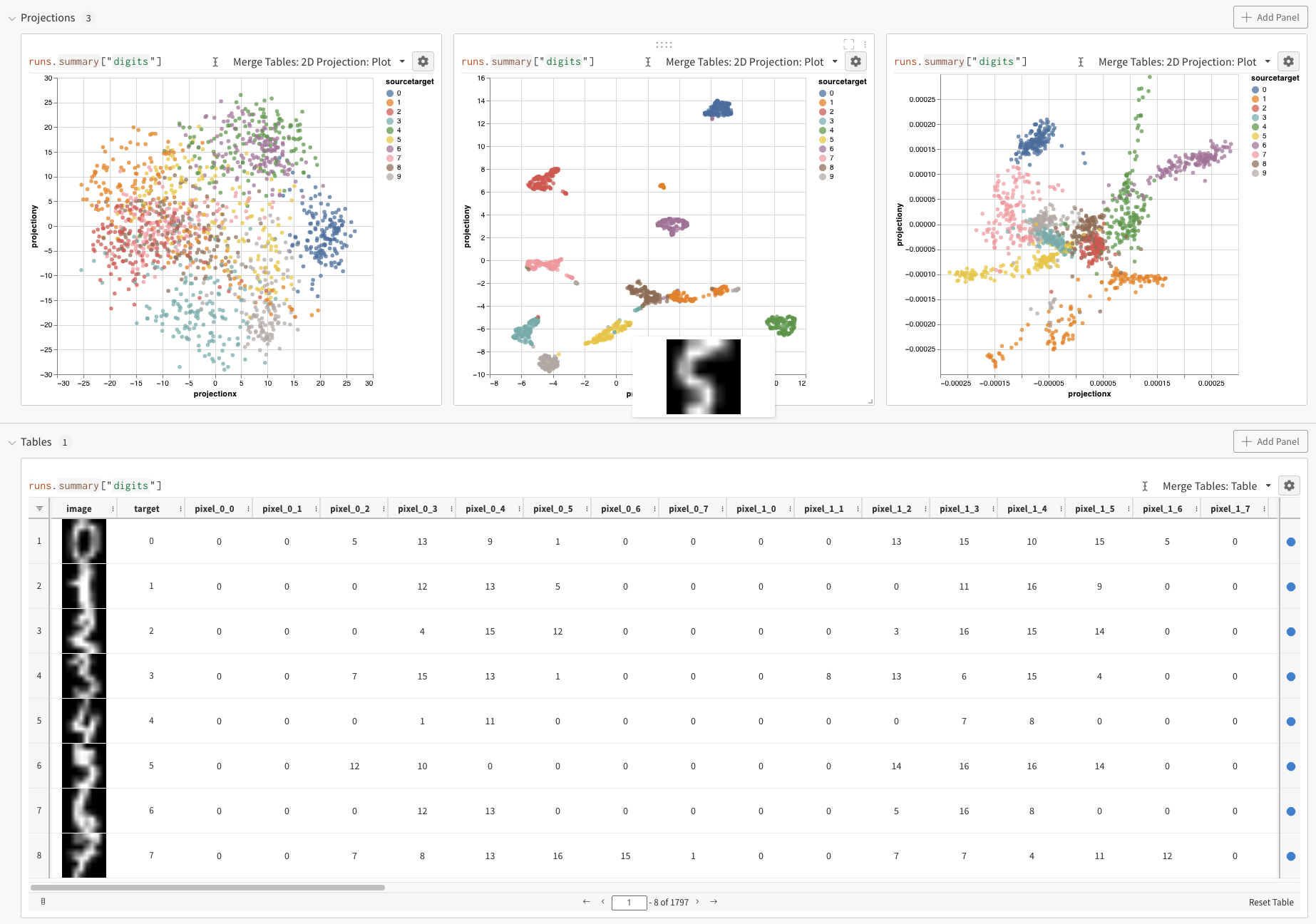
While the above example shows the basic mechanics of logging embeddings, typically you are working with many more dimensions and samples. Let’s consider the MNIST Digits dataset (UCI ML hand-written digits datasets) made available via SciKit-Learn. This dataset has 1797 records, each with 64 dimensions. The problem is a 10 class classification use case. We can convert the input data to an image for visualization as well.
After running the above code, again we are presented with a Table in the UI. By selecting 2D Projection we can configure the definition of the embedding, coloring, algorithm (PCA, UMAP, t-SNE), algorithm parameters, and even overlay (in this case we show the image when hovering over a point). In this particular case, these are all “smart defaults” and you should see something very similar with a single click on 2D Projection. (Click here to interact with this example).
Logging Options
You can log embeddings in a number of different formats:
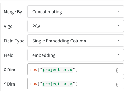
- Single Embedding Column: Often your data is already in a “matrix”-like format. In this case, you can create a single embedding column - where the data type of the cell values can be
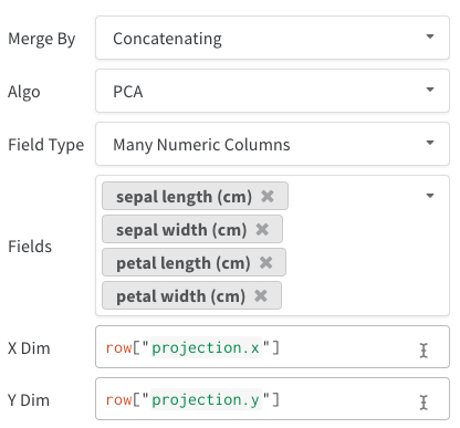
list[int],list[float], ornp.ndarray. - Multiple Numeric Columns: In the above two examples, we use this approach and create a column for each dimension. We currently accept python
intorfloatfor the cells.
Furthermore, just like all tables, you have many options regarding how to construct the table:
- Directly from a dataframe using
wandb.Table(dataframe=df) - Directly from a list of data using
wandb.Table(data=[...], columns=[...]) - Build the table incrementally row-by-row (great if you have a loop in your code). Add rows to your table using
table.add_data(...) - Add an embedding column to your table (great if you have a list of predictions in the form of embeddings):
table.add_col("col_name", ...) - Add a computed column (great if you have a function or model you want to map over your table):
table.add_computed_columns(lambda row, ndx: {"embedding": model.predict(row)})
Plotting Options
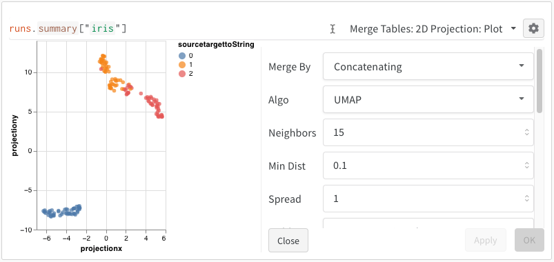
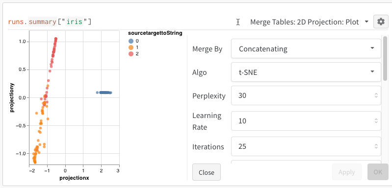
After selecting 2D Projection, you can click the gear icon to edit the rendering settings. In addition to selecting the intended columns (see above), you can select an algorithm of interest (along with the desired parameters). Below you can see the parameters for UMAP and t-SNE respectively.
Feedback
Was this page helpful?
Glad to hear it! If you have more to say, please let us know.
Sorry to hear that. Please tell us how we can improve.