- Compare two W&B Tables logged as artifact versions to analyze changes in your data or model performance.
- Understand higher-level patterns in your data
- View how values you log to a table change throughout your runs.
W&B Tables posses the following behaviors:
- Stateless in an artifact context: any table logged alongside an artifact version resets to its default state after you close the browser window
- Stateful in a workspace or report context: any changes you make to a table in a single run workspace, multi-run project workspace, or Report persists.
Table comparison options
Compare two tables with a merged view or a side-by-side view. For example, the image below demonstrates a table comparison of MNIST data.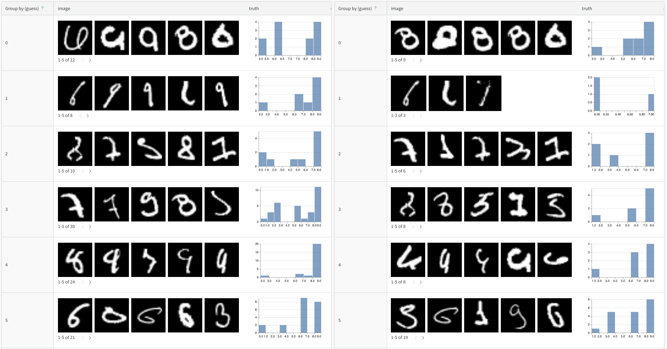
- Go to your project in the W&B App.
- Select the artifacts icon in the project sidebar.
- Select an artifact version.
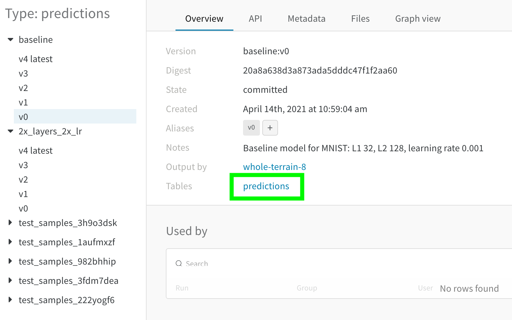
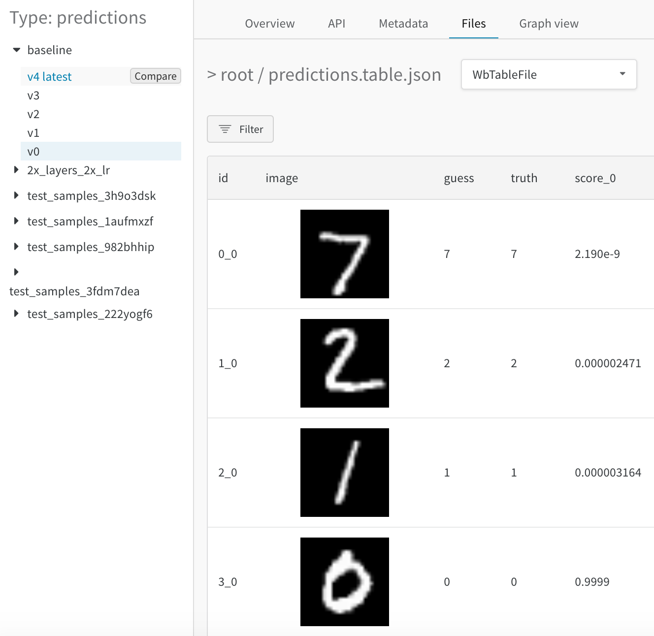
- Hover over the second artifact version you want to compare in the sidebar and click Compare when it appears. For example, in the image below we select a version labeled as “v4” to compare to MNIST predictions made by the same model after 5 epochs of training.
Merged view
Initially you see both tables merged together. The first table selected has index 0 and a blue highlight, and the second table has index 1 and a yellow highlight. View a live example of merged tables here.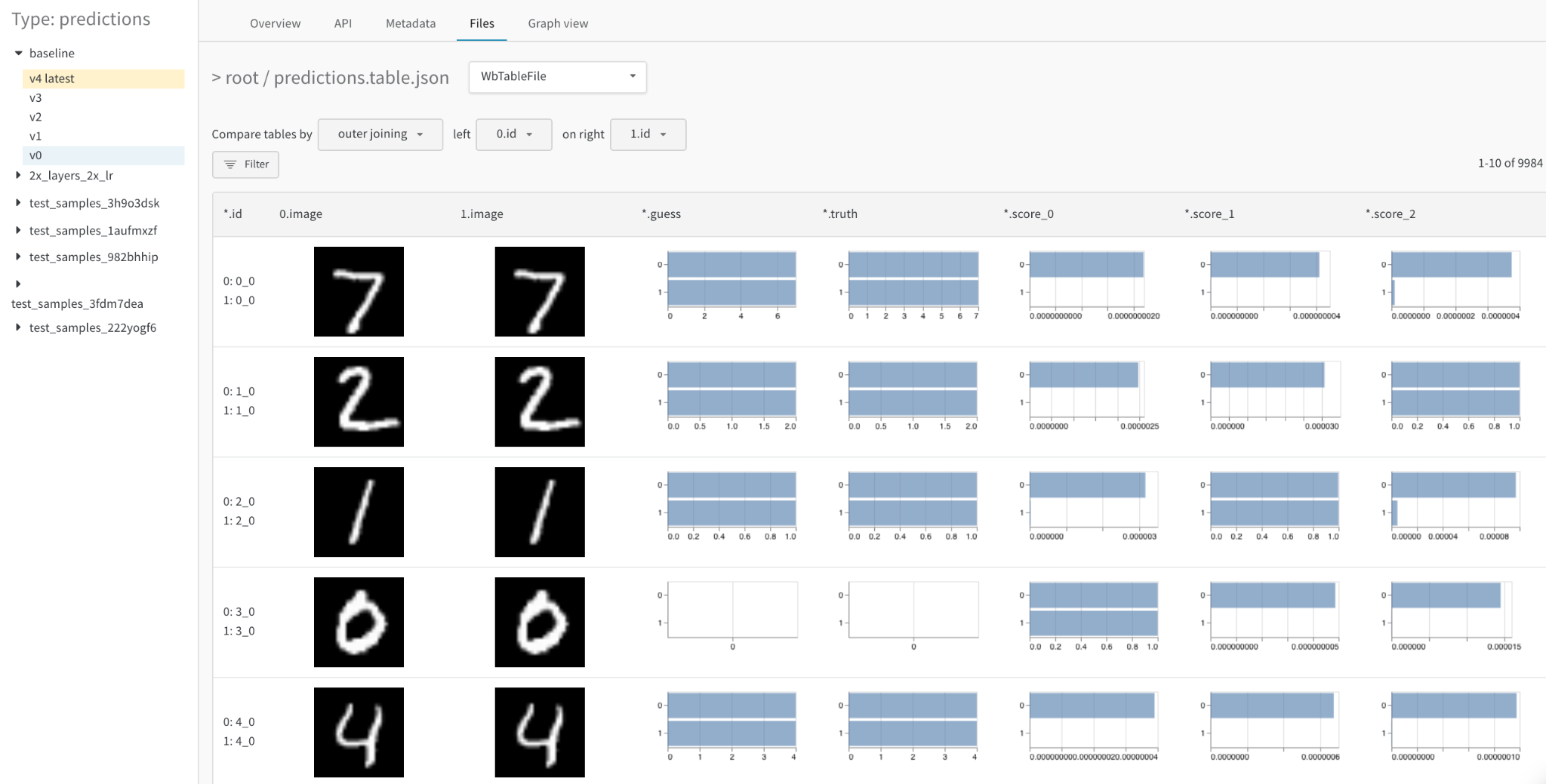
- choose the join key: use the dropdown at the top left to set the column to use as the join key for the two tables. Typically this is the unique identifier of each row, such as the filename of a specific example in your dataset or an incrementing index on your generated samples. Note that it’s currently possible to select any column, which may yield illegible tables and slow queries.
- concatenate instead of join: select “concatenating all tables” in this dropdown to union all the rows from both tables into one larger Table instead of joining across their columns
- reference each Table explicitly: use 0, 1, and * in the filter expression to explicitly specify a column in one or both table instances
- visualize detailed numerical differences as histograms: compare the values in any cell at a glance
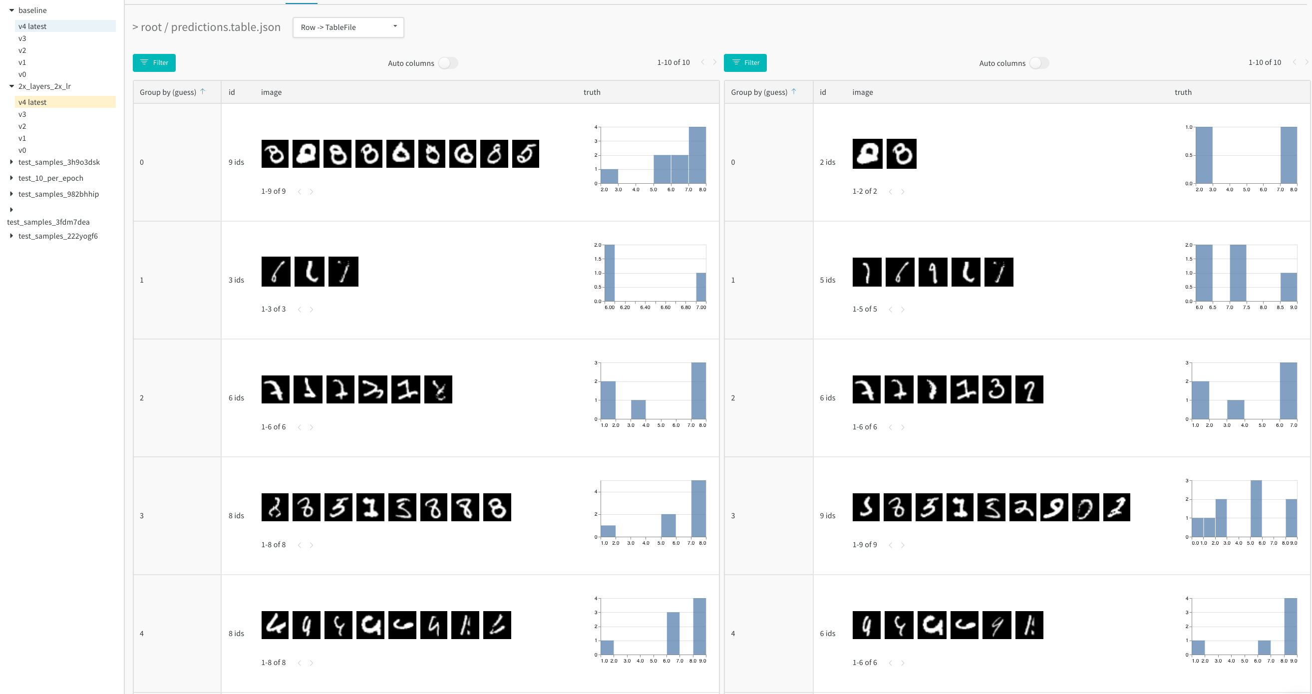
Side-by-side view
To view the two tables side-by-side, change the first dropdown from “Merge Tables: Table” to “List of: Table” and then update the “Page size” respectively. Here the first Table selected is on the left and the second one is on the right. Also, you can compare these tables vertically as well by clicking on the “Vertical” checkbox.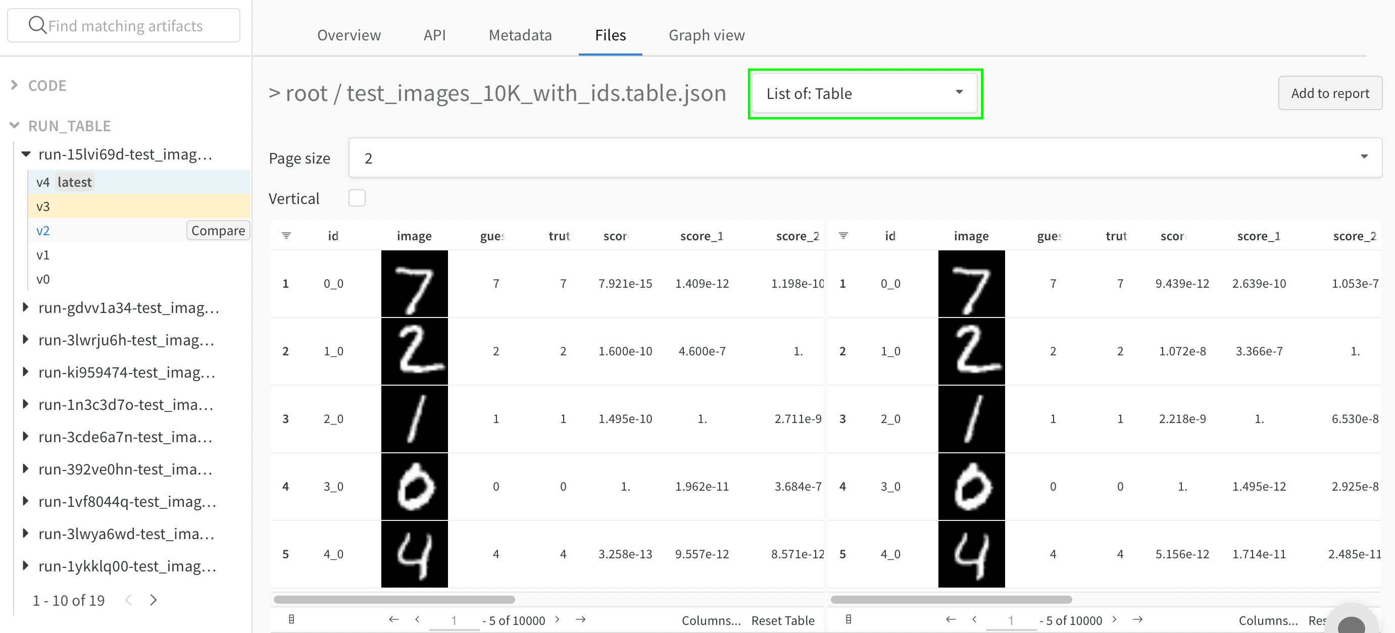
- compare the tables at a glance: apply any operations (sort, filter, group) to both tables in tandem and spot any changes or differences quickly. For example, view the incorrect predictions grouped by guess, the hardest negatives overall, the confidence score distribution by true label, etc.
- explore two tables independently: scroll through and focus on the side/rows of interest
Compare artifacts
Compare two W&B Tables logged as artifact versions to analyze changes in your data or model performance. Use the merged view or side-by-side view to compare the tables.Compare tables across time
Log a table in an artifact for each meaningful step of training to analyze model performance over training time. For example, you could log a table at the end of every validation step, after every 50 epochs of training, or any frequency that makes sense for your pipeline. Use the side-by-side view to visualize changes in model predictions.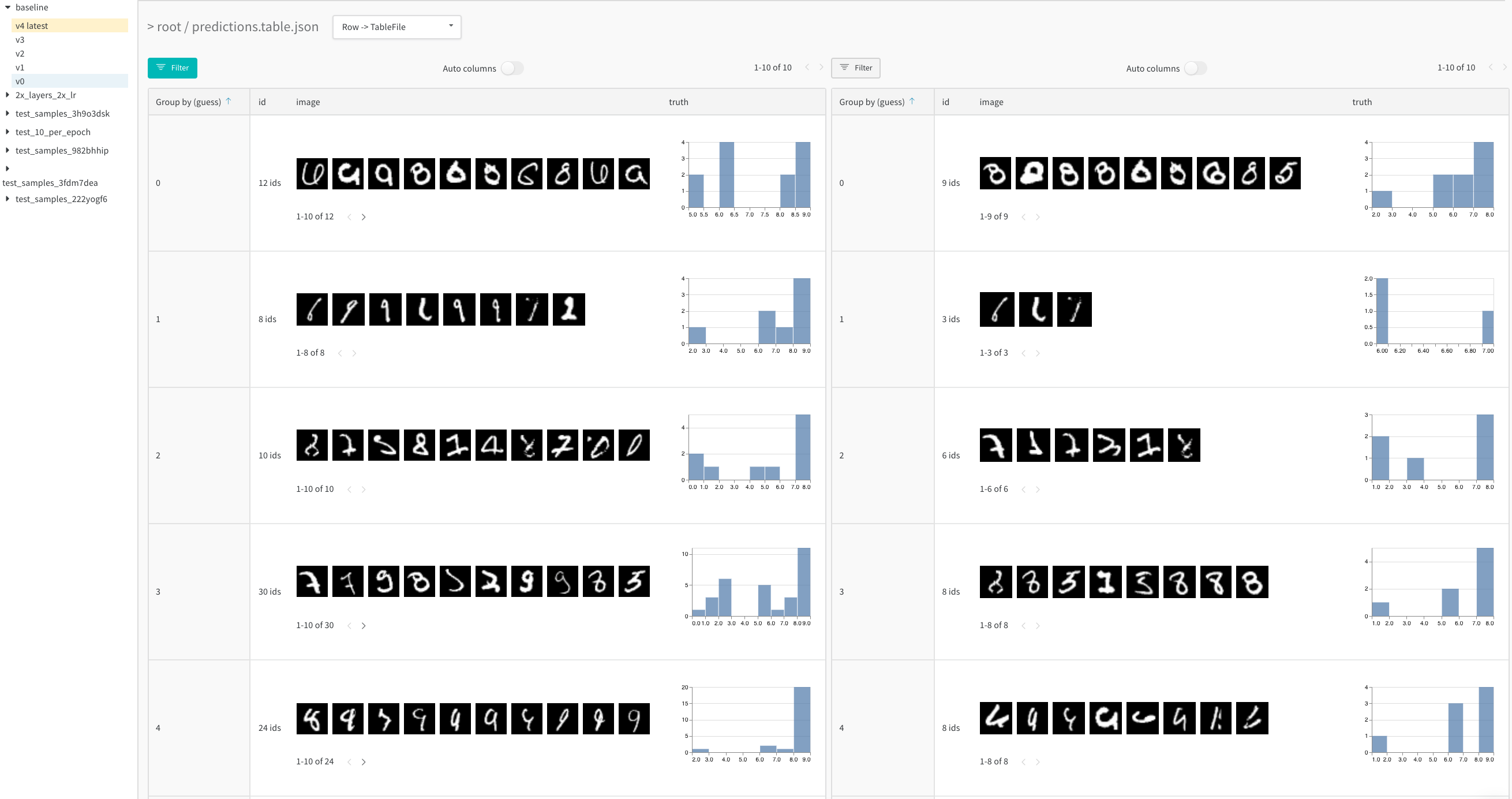
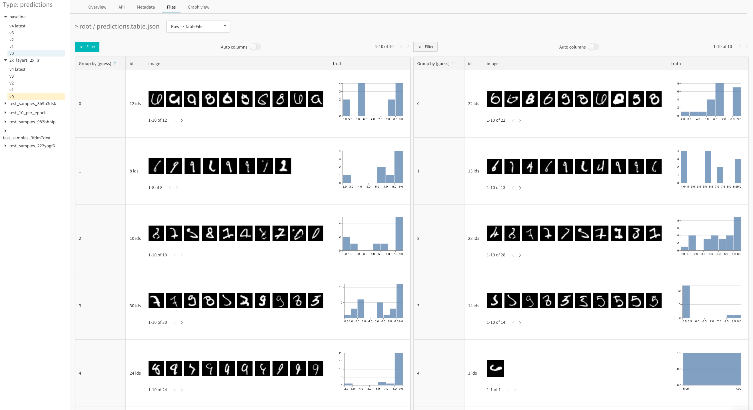
Compare tables across model variants
Compare two artifact versions logged at the same step for two different models to analyze model performance across different configurations (hyperparameters, base architectures, and so forth). For example, compare predictions between abaseline and a new model variant, 2x_layers_2x_lr, where the first convolutional layer doubles from 32 to 64, the second from 128 to 256, and the learning rate from 0.001 to 0.002. From this live example, use the side-by-side view and filter down to the incorrect predictions after 1 (left tab) versus 5 training epochs (right tab).
- 1 training epoch
- 5 training epochs
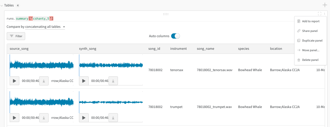
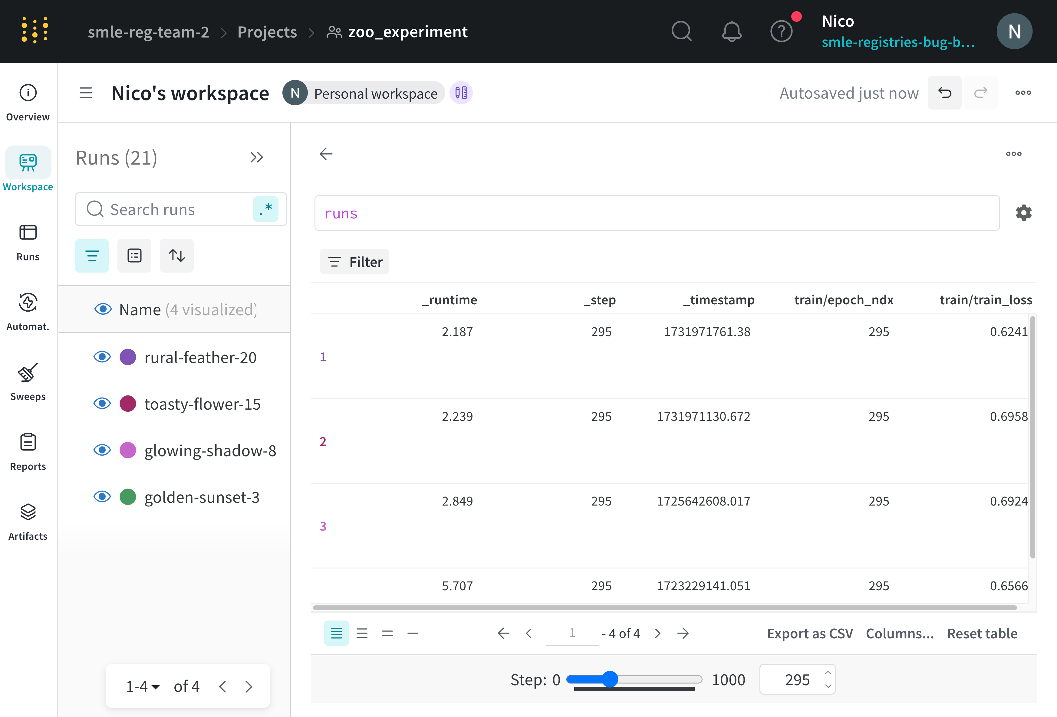
Visualize how values change throughout your runs
View how values you log to a table change throughout your runs with a step slider. Slide the step slider to view the values logged at different steps. For example, you can view how the loss, accuracy, or other metrics change after each run. The slider uses a key to determine the step value. The default key for the slider is_step, a special key that W&B automatically logs for you. The _step key is an integer that increments by 1 each time you call wandb.Run.log() in your code.
To add a step slider to a W&B Table:
- Navigate to your project’s workspace.
- Click Add panel in the top right corner of the workspace.
- Select Query panel.
- Within the query expression editor, select
runsand press Enter on your keyboard. - Click the gear icon to view the settings for the panel.
- Set Render As selector to Stepper.
- Set Stepper Key to
_stepor the key to use as the unit for the step slider.
Custom step key
The step key can be any numeric metric that you log in your runs as the step key, such asepoch or global_step. When you use a custom step key, W&B maps each value of that key to a step (_step) in the run.
This table shows how a custom step key epoch maps to _step values for three different runs: serene-sponge, lively-frog, and vague-cloud. Each row represents a call to wandb.Run.log() at a particular _step in a run. The columns show the corresponding epoch values, if any, that were logged at those steps. Some _step values are omitted to save space.
The first time wandb.Run.log() was called, none of the runs logged an epoch value, so the table shows empty values for epoch.
Now, if the slider is set to
epoch = 1, the following happens:
vague-cloudfindsepoch = 1and returns the value logged at_step = 5lively-frogfindsepoch = 1and returns the value logged at_step = 4serene-spongefindsepoch = 1and returns the value logged at_step = 2
epoch = 9:
vague-cloudalso doesn’t logepoch = 9, so W&B uses the latest prior valueepoch = 3and returns the value logged at_step = 20lively-frogdoesn’t logepoch = 9, but the latest prior value isepoch = 5so it returns the value logged at_step = 20serene-spongefindsepoch = 9and return the value logged at_step = 18
Save your view
Tables you interact with in the run workspace, project workspace, or a report automatically saves their view state. If you apply any table operations then close your browser, the table retains the last viewed configuration when you next navigate to the table.Tables you interact with in the artifact context remains stateless.
- Select the action () menu in the top right corner of your workspace visualization panel.
- Select either Share panel or Add to report.